Experiments

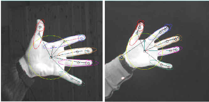
As an illustration of our approach, let's first return to the example shown in Figure 1, where we observed the need for many-to-many matching. The results of applying our method to the these two images is shown in Figure 5, in which many-to-many feature correspondences have been colored the same. For example, a set of blobs and ridges describing a finger in the left image is mapped to a set of blobs in ridges on the corresponding finger in the right image.

Figure 5: Applying our algorithm to the images in Figure 1. Many-to-many feature correspondences have been colored the same.

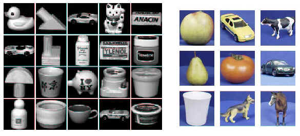
To provide a more comprehensive evaluation, we tested our framework on two separate image libraries, the Columbia University COIL-20 (20 objects, 72 views per object) and the ETH Zurich ETH-80 (8 categories, 10 exemplars per category, 41 views per exemplar). For each view, we compute a multi-scale blob decomposition, using the algorithm described in [19]. Next, we compute the tree metric corresponding to the complete edge-weighted graph defined on the regions of the scale-space decomposition of the view. The edge weights are computed as a function of the distances between the centroids of the regions in the scale-space representation. Finally, each tree is embedded into a normed space of prescribed dimension. This procedure results in two databases of weighted point sets, each point set representing an embedded graph.

Figure 6: Views of sample objects from the Columbia University Image Library (COIL-20) and the ETH Zurich (ETH-80) Image Set.

For the COIL-20 database, we begin by removing 36 (of the 72) representative views of each object (every other view), and use these removed views as queries to the remaining view database (the other 36 views for each of the 20 objects). We then compute the distance between each ``query'' view and each of the remaining database views, using our proposed matching algorithm. Ideally, for any given query view $i$ of object $j$, $v_{i,j}$, the matching algorithm should return either $v_{i+1,j}$ or $v_{i-1,j}$ as the closest view. We will classify this as a correct matching. Based on the overall matching statistics, we observe that in all but $4.8\%$ of the experiments, the closest match selected by our algorithm was a neighboring view. Moreover, among the mismatches, the closest view belonged to the same object in $81.02\%$ of the cases. In comparison to the many-to-many matching algorithm based on PCA embedding [7] for a similar setup, the new procedure showed an improvement of 5.5%. It should be pointed out that these results can be considered worst case for two reasons. First, the original 72 views per object sampling resolution was tuned for an eigenimage approach. Given the high similarity among neighboring views, it could be argued that our matching criterion is overly harsh, and that perhaps a measure of ``viewpoint distance'', i.e., ``how many views away was the closest match'' would be less severe. In any case, we anticipate that with fewer samples per object, neighboring views would be more dissimilar, and our matching results would improve. Second, and perhaps more importantly, many of the objects are symmetric, and if a query neighbor has an identical view elsewhere on the object, that view might be chosen (with equal distance) and scored as an error. Many of the objects in the database are rotationally symmetric, yielding identical views from each viewpoint. For the ETH-80 database, we chose a subset of 32 objects (4 from each of the 8 categories) with full sampling (41 views) per object. For each object, we removed each of its 41 views from the database, one view at a time, and used the removed view as a query to the remaining view database. We then computed the distance between each query view and each of the remaining database views. The criteria for correct classification was similar to the COIL-20 experiment. Our experiments showed that in all but $6.2\%$ of the experiments, the closest match selected by our algorithm was a neighboring view. Among the mismatches, the closest view belonged to the same object in $77.19\%$ of the cases, and the same category in $96.27\%$ of the cases. Again, these results can be considered worst case for the same reasons discussed above for the COIL-20 experiment. Both the embedding and matching procedures can accommodate local perturbation, due to noise and occlusion, because path partitions provide locality. If a portion of the graph is corrupted, the projections of unperturbed nodes will not be affected. Moreover, the matching procedure is an iterative process driven by flow optimization which, in turn, depends only on local features, and is thereby unaffected by local perturbation. To demonstrate the framework's robustness, we performed four perturbation experiments on the COIL-20 database. The experiments are identical to the COIL-20 experiment above, except that the query graph was perturbed by adding/deleting 5%, 10%, 15%, and 20% of its nodes (and their adjoining edges). The results are shown in Table 1, and reveal that the error rate increases gracefully as a function of increased perturbation.

Table 1: Recognition rate as a function of increasing perturbation. Note that the baseline recognition rate (with no perturbation) is 95.2%

PERTURBATION	5%	10%	15%	20%
RECOGNITION RATE	91.07%	88.13%	83.68%	77.72%