Hannes Kruppa and Bernt Schiele
Perceptual Computing and Computer Vision Group
ETH Zurich, Switzerland
{kruppa,schiele}@inf.ethz.ch
http://www.vision.ethz.ch/pccv
Mutual information has been used previously in computer vision, for example in image registration [4] or in audio-visual speech acquisition [3]. As detailed below, mutual information can be used to measure the mutual agreement between two object models. In order to combine multiple models a hierarchy of pairwise model combinations is used.
The mutual information of two random variables ![]() and
and ![]() with a
joint probability mass function
with a
joint probability mass function ![]() and marginal probability mass
functions
and marginal probability mass
functions ![]() and
and ![]() is defined as [1]:
is defined as [1]:
Here, the probabilities in expression 1 can be directly
derived from a pair of distinct visual object models. To undermine the
relevance of mutual information in the context of object model
combination, we briefly refer to the well-known Kullback-Leibler
divergence. The KL-divergence between a probability mass function
![]() and a distinct probability mass function
and a distinct probability mass function ![]() is defined
as:
is defined
as:
 |
(2) |
Although the Kullback-Leibler divergence (also called relative entropy or
information divergence) is not symmetric and does not satisfy the triangle
inequality, it is often useful to think of it as a ``distance'' between
distributions [1].
By defining
![]() the mutual
information can be written as the KL-divergence between
the mutual
information can be written as the KL-divergence between ![]() and
and
![]() :
:
| (3) |
Mutual information therefore measures the ``distance'' between the joint
probability ![]() and the probability
and the probability
![]() , which is
the joint probability under the assumption of
independence. Conversely, it measures mutual dependency or the amount
of information one object model contains about another. As a result
mutual information can be used to measure mutual agreement
between object models.
, which is
the joint probability under the assumption of
independence. Conversely, it measures mutual dependency or the amount
of information one object model contains about another. As a result
mutual information can be used to measure mutual agreement
between object models.
In the following we assume that for each subregion of the input image,
each model determines the probability that the object of interest is
either present or absent. This representation is very general and can
be satisfied by nearly any object model. ![]() is calculated based
on the first object model and covers two cases, namely the presence of
the object
is calculated based
on the first object model and covers two cases, namely the presence of
the object ![]() or its absence
or its absence
![]() ,
respectively. The probability
,
respectively. The probability ![]() is derived from the second object
model analogously, also with the two described cases. Finally, for the
joint probability
is derived from the second object
model analogously, also with the two described cases. Finally, for the
joint probability ![]() both models and all four cases are taken
into account.
both models and all four cases are taken
into account.
Typically, the object of interest can be associated with a
characteristic parameter range of an object model. For
example, in the case of a color model, the parameter range may be
given by a particular subspace of the total color-space. Note that
each parameter configuration results in distinct probabilities ![]() and
and ![]() and consequently, in a distinct mutual information
value. Therefore, one can determine a configuration
and consequently, in a distinct mutual information
value. Therefore, one can determine a configuration
![]() which maximizes mutual agreement
between the employed models and the input data by maximizing the
mutual information over the object-specific joint parameter space:
which maximizes mutual agreement
between the employed models and the input data by maximizing the
mutual information over the object-specific joint parameter space:
| (4) |
with ![]() and
and ![]() describing the object-specific parameter
space of a model pair. For example the parameters of the facial shape
model in the experiments described below are the size and the location
of the face within the image. By maximizing mutual information with a
second, complementary face model the algorithm detects and locates
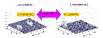
faces in the image. Figure 1 illustrates this concept.
describing the object-specific parameter
space of a model pair. For example the parameters of the facial shape
model in the experiments described below are the size and the location
of the face within the image. By maximizing mutual information with a
second, complementary face model the algorithm detects and locates
faces in the image. Figure 1 illustrates this concept.
 |
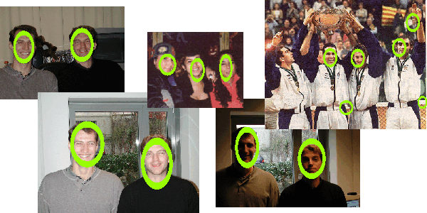
In order to combine multiple models a hierarchy of pairwise model combinations is used. At each stage the algorithm computes a ranking of parameter configurations which maximize mutual information. This ranking is then used as input for the next stage in the hierarchy where mutual information can be used again to find the best combined parameter configurations. The resulting algorithm is modular and can be easily extended to new object models. The hierarchical concept is depicted in figure 2 which shows the architecture used for face detection (see figures 3, 4, 5). In this case study, the following three object models are combined pairwise in order to detect human faces: a skin color model, a shape model and a template matcher. In stage one the probability maps are calculated based on the color model and the template matcher. Stage two combines the color model with the facial shape model by maximizing mutual information. The template matcher and the facial shape model are also combined in stage two. Finally stage three combines both results again by maximizing mutual information.
Obviously other groupings would be meaningful as well. The proposed grouping however ensures that the combined hypotheses on stage two can be represented as a single condensed region of probabilities. This will be further explained in the next sections. Also, it would be possible to combine all models in a single maximization step. However, using pairwise combinations enables the definition of separate and independent parameter constraints for each pair which reduces the size of the joint parameter space and therefore speeds up sampling.
 |
 |
 |
 |