Accuracy vs. Efficiency Trade-offs in Optical Flow Algorithms
Hongche Liu, Tsai-Hong Hong, Martin Herman, and Rama Chellappa
hongche@etak.com, hongt@cme.nist.gov, herman@cme.nist.gov, rama@cfar.umd.edu
Intelligent Systems Division, National Institute of Standards and Technology (NIST)
Blg. 220, Rm B124, Gaithersburg, MD 20899
Center for Automation Research/Department of Electrical Engineering,
Abstract
There have been two thrusts in the development of optical flow algorithms. One has emphasized higher accuracy; the other faster implementation. These two thrusts, however, have been independently pursued, without addressing the accuracy vs. efficiency trade-offs. Although the accuracy-efficiency characteristic is algorithm dependent, an understanding of a general pattern is crucial in evaluating an algorithm as far as real world tasks are concerned, which often pose various performance requirements. This paper addresses many implementation issues that have often been neglected in previous research, including subsampling, temporal filtering of the output stream, algorithms' flexibility and robustness, etc. Their impacts on accuracy and/or efficiency are emphasized. We present a critical survey of different approaches toward the goal of higher performance and present experimental studies on accuracy vs. efficiency trade-offs. The goal of this paper is to bridge the gap between the accuracy and the efficiency-oriented approaches.
1. Introduction
Whether the results of motion estimation are used in robot navigation, object tracking, or some other applications, one of the most compelling requirements for an algorithm to be effective is adequate speed. No matter how accurate an algorithm may be, it is not useful unless it can output the results within the necessary response time for a given task. On the other hand, no matter how fast an algorithm runs, it is useless unless it computes motion sufficiently accurately and precisely for subsequent interpretations.
Both accuracy and efficiency are important as far as real world applications are concerned. However, recent motion research has taken two approaches in opposite directions. One neglects all considerations of efficiency to achieve the highest accuracy possible. The other trades off accuracy for speed as required by a task. These two criteria could span a whole spectrum of different algorithms, ranging from very accurate but slow to very fast but highly inaccurate. Most existing motion algorithms are clustered at either end of the spectrum. Applications which need a certain combination of speed and accuracy may not find a good solution among these motion algorithms. To evaluate an algorithm for practical applications, we propose a 2-dimensional scale where one of the coordinates is accuracy and the other is time efficiency. In this scale, an algorithm that allows different parameter settings generates an accuracy-efficiency (AE) curve, which will assist users in understanding its operating range (accuracy-efficiency trade-offs) in order to optimize the performance.
In evaluating the accuracy-efficiency trade-offs, we also consider implementation issues such as subsampling, temporal filtering and their effects on both accuracy and speed.
Since Barron, et al. have published a detailed report [4] regarding accuracy aspects of optical flow algorithms, we start here with a survey of real-time implementations.
2. Previous Work on Real-Time Implementations
Regarding the issue of speed, there is a prevailing argument in most motion estimation literature that with more advanced hardware in the near future, the techniques could be implemented to run at frame rate [4] . In a recent report, many existing algorithms' speeds (computing optical flow for the diverging trees sequence) are compared and compiled in a tabular form [5] . We use the data from this table and calculate the time (in years) it may take for these algorithms to achieve frame rate, assuming computing power doubles every year [28] . This result is displayed in Table 1 . Note that some algorithms can take up to 14 years (from when the table was compiled) to achieve frame rates. This would drastically limit the potential of such algorithms for many practical applications over the next decade.
|
Execution time (min:sec) (from [5] ) |
||||||
There have been numerous attempts to realize fast motion algorithms. There are two major approaches: the hardware approach and the algorithmic approach. They are summarized in Table 2 and Table 3 given below and elaborated in the following paragraphs.
|
Connection machine [6] [26] [37] [39] , Parsytec transputer [32] and hybrid pyramidal vision machine (AIS-4000 and CSA transputer) [11] |
||
|
Vision Chips: gradient method [23] [34] , correspondence method [10] [33] and biological receptive field design [12] [22] |
||
|
Non-Vision Chips: analog neural networks [17] digital block matching technique [3] [15] [38] |
|
tracking [1] [20] [24] , computing time-to-contact (and hence obstacle avoidance) [9] and segmentation [32] |
||
|---|---|---|
|
constraint on motion velocity [8] , constraint on projection [40] |
||
|
1-D spatial search [2] , separable filter design (Liu's algorithm [18] ) |
The hardware approach uses specialized hardware to achieve real-time performance. There have been three categories of specialized hardware employed for motion estimation: parallel computers, specialized image processing hardware and dedicated VLSI chips. The hardware approach generally suffers from high cost and low precision.
The most popular algorithmic method is to compute sparse feature motion. Recent advances in this approach have enabled versatile applications including tracking [1] [20] [24] , computing time-to-contact (and hence obstacle avoidance) [9] and even segmentation [32] , which were believed to be better handled with dense data. However, in order to interpret the scenes with only sparse features, these algorithms need to use extensive temporal information (e.g., recursive least squares, Kalman filtering), which is time-consuming. Therefore, either the speed is not satisfactory [1] or they need to run on special hardware to achieve high speed [9] [20] [32] .
Another method is to constrain the motion estimation to a more tractable problem. For example, images can be subsampled so that the maximum velocity is constrained to be less than 1 pixel per frame. Therefore, a correlation method [8] can simply perform temporal matching in linear time instead of spatial searching in quadratic time. Another technique is to use a different projection. For example, any 3-D vertical line appears as a radial line in a conic projected image. This fact has been exploited for real-time navigation [40] .
Another elegant idea is to work on efficient design and implementation of the flow estimation algorithm. The main goal of this approach is to reduce the computational complexity. Suppose the image size is  and the maximum motion velocity is
  . Traditional correlation algorithms performing spatial search or gradient-based algorithms using 2-D filters have the complexity
  . Several recent spatio-temporal filter based methods
[13]
[14]
even have
. Several recent spatio-temporal filter based methods
[13]
[14]
even have  complexity. However, some recent algorithms have achieved
  complexity. These include a correlation-based algorithm that uses 1-D spatial search
[2]
and a gradient-based algorithm
[18]
that exploits filter separability. These algorithm are so efficient that they achieve satisfactory rate on general purpose workstations or microcomputers.
complexity. These include a correlation-based algorithm that uses 1-D spatial search
[2]
and a gradient-based algorithm
[18]
that exploits filter separability. These algorithm are so efficient that they achieve satisfactory rate on general purpose workstations or microcomputers.
3. Accuracy vs. Efficiency Trade-offs
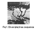
Although real-time is often used to mean video frame rates, in this paper, real-time is loosely defined as sufficiently fast for interactions with humans, robots or imaging hardware. The following subsections discuss the issues that are only of interest when one is concerned about both accuracy and speed. All the experiments illustrating our discussions are done on the diverging tree sequence [4] .
Accuracy-efficiency curve
If a motion algorithm is intended to be applied in a real-world task, the overall performance, including accuracy and efficiency, should be evaluated. Analogous to the use of electronic devices (e.g., transistor), without the knowledge of an algorithm's full operating range and characteristics, one may fail to use it in its optimal condition. Using accuracy (or error) as one coordinate and efficiency (or execution time) as the other, we propose the use of a 2-D accuracy-efficiency (AE) curve to characterize an algorithm's performance. This curve is generated by setting parameters in the algorithm to different values.
For correlation methods, the template window size and the search window size are common parameters. For gradient methods, the (smoothing or differentiation) filter size is a common parameter. More complex algorithms may have other parameters to consider. The important thing is to characterize them in a quantitative way.
For optical flow, accuracy has been extensively researched in Barron, et al.
[4]
. We will use the error measure in
[4]
, that is, the angle error between computed flow  and the ground truth flow
  , as one quantitative criterion. For efficiency, we use throughput (number of output frames per unit time) or its reciprocal (execution time per output frame) as the other quantitative criterion.
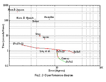
In the 2-D performance diagram depicted below (
Fig 2.
), the  axis represents the angle error; the
  axis represents the execution time. A point in the performance diagram corresponds to a certain parameter setting. The closer the performance point is to the origin (small error and low execution time), the better the algorithm is. An algorithm with different parameter settings spans a curve, usually of negative slope. The distance from the origin to the AE curve represents the algorithm's AE performance. In
See 2-D performance diagram
, there are two AE curves and several points
1
. It can be seen that some algorithms (e.g., Fleet & Jepson
[13]
) may be very accurate but very slow while some algorithms (e.g., Camus
[8]
) may be very fast but not very accurate. In terms of AE performance, Liu, et al.'s algorithm
[18]
is most flexible and effective because the curve is closest to the origin. It is also interesting to find that Liu, et al.'s curve
[18]
is relatively horizontal and Camus's
[8]
curve is relatively vertical they intersect each other.
axis represents the execution time. A point in the performance diagram corresponds to a certain parameter setting. The closer the performance point is to the origin (small error and low execution time), the better the algorithm is. An algorithm with different parameter settings spans a curve, usually of negative slope. The distance from the origin to the AE curve represents the algorithm's AE performance. In
See 2-D performance diagram
, there are two AE curves and several points
1
. It can be seen that some algorithms (e.g., Fleet & Jepson
[13]
) may be very accurate but very slow while some algorithms (e.g., Camus
[8]
) may be very fast but not very accurate. In terms of AE performance, Liu, et al.'s algorithm
[18]
is most flexible and effective because the curve is closest to the origin. It is also interesting to find that Liu, et al.'s curve
[18]
is relatively horizontal and Camus's
[8]
curve is relatively vertical they intersect each other.
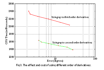
The AE curve is also useful in understanding the effect and cost of certain types of processing. For example, See The effect and cost of using different order of derivatives. shows the effect and cost of using different orders of image derivatives in Liu, et al.'s algorithm. The trade-off is clearer in this example. Using only up to second order derivatives saves 50% in time while sacrificing 85% in accuracy.
Subsampling effect
The computational complexity of an optical flow algorithm is usually proportional to the image size. However, an application may not need the full resolution of the digitized image. An intuitive idea to improve the speed is to subsample the images. Subsampling an image runs the risk of undersampling below the Nyquist frequency, resulting in aliasing, which can confuse motion algorithms. To avoid aliasing, the spatial sampling distance must be smaller than the scale of image texture and the temporal sampling period must be shorter than the scale of time. That is, the image intensity pattern must evidence a phase shift that is small enough to avoid phase ambiguity [30] .
Subsampling should be avoided on an image sequence with high spatial frequency and large motion. The aliasing problem can be dealt with by smoothing (low-pass filtering) before subsampling. However, since smoothing is done on the original images and the computational cost is proportional to the original image size, the advantage of subsampling is lost.
Aliasing is not the only problem in subsampling. Object size in subsampled images is reduced quadratically but the object boundaries are reduced linearly (in terms of number of pixels). Hence the density of motion boundaries are higher. This is detrimental to optical flow algorithms in general.
In short, subsampling can improve efficiency but needs a careful treatment.
Temporal processing of the output
Most general purpose optical flow algorithms are still very inefficient and often operate on short "canned" sequences of images. For long image sequences, it is natural to consider the possibility of temporally integrating the output stream to achieve better accuracy.
Temporal filtering is often used in situations where noisy output from the previous stage cannot be reliably interpreted. Successful applications of temporal filtering on the output requires a model (e.g., Gaussian with known variance) for noise (Kalman filtering) or a model (e.g., quadratic function) for the underlying parameters (recursive least squares). Therefore, these methods are often task specific.
A general purpose Kalman filter has been proposed in [31] where the noise model is tied closely to the framework of the method. In this scheme, an update stage requires point-to-point local warping using the previous optical flow field (as opposed to global warping using a polynomial function) in order to perform predictive filtering. It is computationally very expensive and therefore has little prospect of real-time implementation in the near future. So far, Kalman filters and recursive least square filters implemented in real-time are only limited to sparse data points [20] [9] .
We have experimented with a simple, inexpensive temporal processing approach--exponential filtering. We found out that when the noise in the output is high or the output is expected to remain roughly constant, exponential filtering improves accuracy with little computational overhead. However, when the scene or motion is very complex or contains numerous objects, exponential filtering is less likely to improve accuracy.
Flexibility and robustness
It has been pointed out that some motion algorithms achieve higher speed by constraining the input data, e.g., limiting the motion velocity to be less than a certain value, thus sacrificing some flexibility and robustness. Some algorithms optimize the performance for limited situations. For good performance in other situations, users may need to retune several parameters. It is thus important to understand how these constraints or parameter tuning affects the accuracy. Flexibility refers to an algorithm's capability to handle widely varying scenes and motions. Robustness refers to resistance to noise. These two criteria prescribe an algorithm's applicability to general tasks.
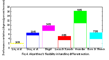
To evaluate an algorithm's flexibility, we have conducted the following simple experiment. A new image sequence is generated by taking every other frame of the diverging trees sequence. The motion in the new sequence will be twice as large as that in the original sequence. We then run algorithms on the new sequence using the same parameter setting as on the original sequence and compare the errors in the two outputs. A flexible algorithm should yield similarly accurate results, so we observe performance variation rather than absolute accuracy here. See Algorithms's flexibility in handling different motion. illustrates the results. The algorithms' performance variation for these two sequences ranges from 16% (Liu, et al.) to 75% (Horn & Shunck). Fleet and Jepson's algorithm, which has been very accurate, failed to generate nonzero density on the new sequence so is not plotted.
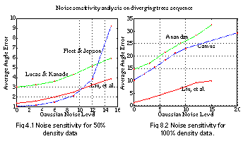
To evaluate an algorithm's noise sensitivity or robustness, we have generated a new diverging tree sequence by adding Gaussian noise of increasing variance and observed the algorithms' performance degradation. See 1 Noise sensitivity for 50% density data illustrates the algorithms' noise sensitivity. Some algorithms (Lucas & Kanade, Liu, et al., Anandan, Camus) have linear noise sensitivity with respect to noise magnitude; some (Fleet and Jepson) show quadratic noise sensitivity.
Output density
With most algorithms, some thresholding is done to eliminate unreliable data and it is hoped that the density is adequate for the subsequent applications. In addition, the threshold value is often chosen arbitrarily (by users who are not experts on the algorithms) without regard to the characteristics of the algorithms. The important characteristics that should be considered are flexibility and robustness to noise. If an algorithm is accurate but not flexible and not robust to noise, then it is better off generating a sparse field because the more data it outputs, the more likely it will contain noisy data. However, the output density should really be determined by the requirements of the subsequent applications. Although dense flow field is ideal, selecting the right density of sufficiently accurate output is perhaps a more practical approach.
Specific experiments in [18] [19] using NASA sequence have shown output density as well as accuracy is the decisive factor in obstacle avoidance.
4. Conclusion
Motion research has typically focused on only accuracy or only speed. We have reviewed many different approaches to achieving higher accuracy or speed and pointed out their difficulties in real world applications. We also have raised the issues of accuracy-efficiency trade-offs resulting from subsampling effects, temporal processing of the output, algorithm flexibility and robustness, and output density. It is only through consideration of these issues that we can address a particular algorithm's applicability to real world tasks. The accuracy-efficiency trade-off issues discussed here are by no means exhaustive. We hope that this initial study can generate more interesting discussions and shed some light on the use of motion algorithms in real world tasks.
References
- Allen, P., Timcenko, A., Yoshimi, B. and Michelman, P., "Automated Tracking and Grasping of a Moving Object with a Robotic Hand-Eye System", IEEE Transactions on Robotics and Automations, vol. 9, no. 2, pp. 152-165, 1993.
- Ancona, N. and Poggio, T., "Optical Flow from 1-D Correlation: Applications to a Simple Time-to-Crash Detector", Proceedings of IEEE International Conference on Computer Vision, Berlin, Germany, pp. 209-214, 1993.
- Artieri, A. and Jutand, F., "A Versatile and Powerful Chip for Real-Time Motion Estimation", Proceedings of IEEE International Conference on Acoustics, Speech, and Signal Processing, Glasgow, UK, pp. 2453-2456, 1989.
- Barron, J. L., Fleet, D. J. and Beauchemin, S. S., "Performance of Optical Flow Techniques", International Journal of Computer Vision, vol. 12, no. 1, pp. 43-77, 1994.
- Bober, M. and Kittler, J., "Robust Motion Analysis", Proceedings of IEEE Conference on Computer Vision and Pattern Recognition, Seattle, WA, pp. 947-952, 1994.
- Bülthoff, H., Little, J. and Poggio, T., "A Parallel Algorithm for Real-Time Computation of Optical Flow", Nature, vol. 337, pp. 549-553, 1989.
- Camus, T., "Calculating Time-to-Contact Using Real-Time Quantized Optical Flow", NISTIR-5609, Gaithersburg, MD, 1995.
- Camus, T., "Real-Time Quantized Optical Flow", Proceedings of IEEE Conference on Computer Architectures for Machine Perception, Como, Italy, 1995.
- Coombs, D., Herman M., Hong T. and Nashman, M., "Real-time Obstacle Avoidance Using Central Flow Divergence and Peripheral Flow", Proceedings of IEEE International Conference on Computer Vision, Cambridge, MA, 1995.
- Delbruck, T., "Silicon Retina with Correlation-Based Velocity-Tuned Pixels", IEEE Transactions on Neural Networks, vol. 4, no. 3, pp. 529-541, 1993.
- Ens, J. and Li, Z.N., "Real-Time Motion Stereo", Proceedings of IEEE Conference on Computer Vision and Pattern Recognition, pp.130-135, New York, NY, 1993.
- Etienne-Cummings, R., Fernando, S.A., Van der Spiegel, J. and Mueller, P., "Real-Time 2D Analog Motion Detector VLSI Circuit", Proceedings of IEEE International Joint Conference on Neural Networks, vol. 4, pp. 426-431, New York, NY, 1992.
- Fleet, D.J. and Jepson, A.L., "Computation of Component Image Velocity from Local Phase Information", International Journal of Computer Vision, vol. 5, no.1, pp. 77-104, 1990.
- Heeger, D. J., "Optical Flow Using Spatiotemporal Filters", International Journal of Computer Vision, vol. 1, no. 4, pp. 279-302, 1988.
- Inoue, H., Tachikawa, T. and Inaba, M., "Robot Vision System with a Correlation Chip for Real-Time Tracking, Optical Flow and Depth Map Generation", Proceedings IEEE Conference on Robotics and Automation, Nice, France, vol. 2, pp. 1621-1626, 1992.
- Koch, C., Marroquin, J. and Yuille, A., "Analog `Neural' Networks in Early Vision", Proceedings of the National Academy of Sciences, vol. 83, pp. 4263-4267, 1986.
- Lee, J.C., Sheu, B. J., Fang, W.C. and Chellappa, R., "VLSI neuroprocessors for Video Motion Detection", IEEE Transactions on Neural Networks, vol. 4, no. 2, pp. 178-191, 1993.
- Liu, H., Hong, T., Herman, M. and Chellappa, R., "A General Motion Model and Spatio-temporal Filters for Computing Optical Flow", University of Maryland TR -3365, November, 1994; NIST-IR 5539, Gaithersburg MD, January, 1995, to appear in International Journal of Computer Vision.
- Liu, H., "A General Motion Model and Spatio-temporal Filters for 3-D Motion Interpretations", PH.D. Dissertation, University of Maryland, September, 1995.
- Matteucci, P., Regazzani, C.S. and Foresti, G.L., "Real-Time Approach to 3-D Object Tracking in Complex Scenes", Electronics Letters, vol. 30, no. 6, pp. 475-477, 1994.
- Mioni, A., "VLSI Vision Chips Homepage", http://www.eleceng.adelaide.edu.au/Groups/GAAS/Bugeye/visionchips.
- Mioni, A., Bouzerdoum, A., Yakovleff, A., Abbott, D., Kim, O., Eshraghian, K. and Bogner, R.E., "An Analog Implementation of Early Visual Processing in Insects", Proceedings International Symposium on VLSI Technology, Systems, and Applications, pp. 283-287, 1993.
- Moore, A. and Koch C., "A Multiplication Based Analog Motion Detection Chip", Proceedings of the SPIE, vol. 1473, Visual Information Processing: From Neurons to Chips, pp. 66--75, 1991.
- Nashman, M., Rippey, W., Hong, T.-H. and Herman, M., "An Integrated Vision Touch-Probe System for Dimensional Inspection Tasks", NISTIR 5678, National Institute of Standards and Technology, 1995.
- Nelson, R., "Qualitative Detection of Motion by a Moving Observer", Proceedings of the IEEE Conference on Computer Vision and Pattern Recognition, Lahaina, HI, pp. 173-178, 1991.
- Nesi, P., DelBimbo, A.D. and Ben-Tzvi, D. "A Robust Algorithm for Optical Flow Estimation", Computer Vision and Image Understanding, vol. 62, no. 1, pp. 59-68, 1995.
- Nishihara, H.K., "Real-Time Stereo- and Motion-Based Figure Ground Discrimination and Tracking Using LOG Sign Correlation", Conference Record of the Twenty-Seventh Asilomar Conference on Signals, Systems and Computers, vol. 1, pp. 95-100, 1993.
- Patterson, D. and Hennessy, J., "Computer Organization and Design: the Hardware/Software Interface", Morgan Kaufman, San Mateo, CA 1994.
- Rangachar, R., Hong, T.-H., Herman, M., and Luck, R., "Three Dimensional Reconstruction from Optical Flow Using Temporal Integration", Proceedings of SPIE Advances in Intelligent Robotic Systems: Intelligent Robots and Computer Vision, Boston, MA, 1990.
- Schunck, B., "Image Flow Segmentation and Estimation by Constraint Line Clustering", IEEE Transactions on Pattern Analysis and Machine Intelligence, vol. 11, no.10, pp. 1010-1027, 1989.
- Singh, A., "Optical Flow Computation: A Unified Perspective", IEEE Computer Society Press, 1991.
- Smith, S.M., "ASSET-2 Real-Time Motion Segmentation and Object Tracking", Proceedings of the Fifth International Conference on Computer Vision, pp. 237-244, Cambridge, MA, 1995.
- Tanner J. and Mead C., "A Correlating Optical Motion Detector", MIT Advanced Research in VLSI, pp. 57--64, 1984.
- Tanner, J. and Mead, C., "An Integrated Analog Optical Motion Sensor", VLSI Signal Processing II, R.W. Brodersen and H.S. Moscovitz, Eds., pp. 59-87, New York, 1988.
- Waxman, A.M., Wu J. and Bergholm F. "Convected Activation Profiles and Receptive Fields for Real Time Measurement of Short Range Visual Motion", Proceedings of IEEE Conference on Computer Vision and Pattern Recognition, Ann Arbor, MI, pp. 717-723, 1988.
- Weber, J. and Malik, J., "Robust Computation of Optical Flow in a Multi-Scale Differential Framework", Proceedings of the Fourth International Conference on Computer Vision, Berlin, Germany, 1993.
- Weber, J. and Malik, J., "Robust Computation of Optical Flow in a Multi-Scale Differential Framework", International Journal of Computer Vision, vol. 14, pp. 67-81, 1995.
- Weiss, P. and Christensson, B., "Real Time Implementation of Subpixel Motion Estimation for Broadcast Applications", IEE Colloquim on Applications of Motion Compensation, London, UK, no. 128, pp. 7/1-3, 1990.
- Woodfill, J. and Zabin, R., "An Algorithm for Real-Time Tracking of Non-Rigid Objects", Proceedings of the Ninth National Conference on Artificial Intelligence, pp. 718-723, 1991.
- Yagi, Y., Kawato, S. and Tsuji, S., "Real-Time Omnidirectional Image Sensor (COPIS) for Vision-Guided Navigation", IEEE Transactions on Robotics and Automation, vol. 10, no. 1, pp. 11-22, 1994.