


Next: References
Up: Computer Vision IT412
Previous: Solving for the calibration
Subsections
We assume that we are given the 3D coordinate vectors  of N
reference points Mi as well as the 2D retinal coordinates (ui, vi)
of their images. In general, we have at least 6 points, preferably more,
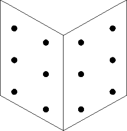
and they are arranged in a special pattern, such as that shown in figure 2.
of N
reference points Mi as well as the 2D retinal coordinates (ui, vi)
of their images. In general, we have at least 6 points, preferably more,
and they are arranged in a special pattern, such as that shown in figure 2.
Figure 2:
The pattern of points on a calibration frame.
 |
There are several methods for obtaining the coefficients of the matrix
C. We will outline both linear and non-linear methods.
Recall that in homogeneous coordinates we have a linear relationship
between the image points mi and the 3D reference points Mi given
by
![\begin{displaymath}
\left[ \begin{array}
{c}
su \\ sv \\ s
\end{array} \righ...
...[ \begin{array}
{c}
X \\ Y \\ Z \\ 1
\end{array} \right]. \end{displaymath}](img47.gif)
Because of the arbitrary scale factor involved, we have set
q34 = 1.
From this equation we can write
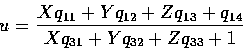
and
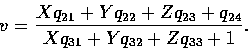
This implies that
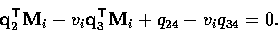
Xq11 + Yq12 + Zq13 + q14 - uXq31 - uYq32 - uZq33 = u
and
Xq21 + Yq22 + Zq23 + q24 - vXq31 - vYq32 - vZq33 = v.
In fact, using the given structure of C, this can be written
in shorthand as
and
We can write this as
|  |
(5) |
where L is a  matrix and q is a
  vector.
We will first solve this system, however, without taking into account
any special structure in the matrix C.
So given a set of N 3D world points and their image coordinates, we
can build up the following matrix equation:
![\begin{displaymath}
\left[ \begin{array}
{ccccccccccc}
X_1 & Y_1 & Z_1 & 1 & 0 ...
... \\ . \\ . \\ . \\ . \\ u_m \\ v_m
\end{array} \right], \end{displaymath}](img55.gif)
where the matrix of knowns is  .
.
With 11 unknowns and each point providing 2 constraint equations, we
need at least six points to solve the equation.
The best least squares estimate of the qij is obtained using the
pseudo-inverse. If we write the equation above as
![\begin{displaymath}[{\bf B}]
[{\bf C}] = [{\bf UV}] \end{displaymath}](img57.gif)
then
![\begin{displaymath}[{\bf C}]
= [{\bf B}]^+[{\bf UV}]. \end{displaymath}](img58.gif)
When the equations are over-constrained, as in our case, the pseudo-inverse
is given by
![\begin{displaymath}[{\bf B}]
^+ = [{\bf B}^{\top}{\bf B}]^{-1}{\bf B}^{\top}. \end{displaymath}](img59.gif)
In general, this matrix equation is very ill-conditioned and care
must be taken in finding its solution.
Let's return now to the formulation given in equation (5). This is just
a system of linear equation and we want to solve for q. Constraints
must be imposed upon q however, to avoid the trivial solution
q = 0, which is not physically significant. It is natural to use the
constraints given to us by the structure of the matrix C, namely
 and
and  . This is done via a technique known as constrained
optimisation, which we will not cover in lectures. Suffice it to say, it
leads to a closed form solution. What is of more interest though, is the
question of the rank of the matrix L, since this leads to an
understanding of how the reference points should be chosen.
. This is done via a technique known as constrained
optimisation, which we will not cover in lectures. Suffice it to say, it
leads to a closed form solution. What is of more interest though, is the
question of the rank of the matrix L, since this leads to an
understanding of how the reference points should be chosen.
We know from standard linear algebra that if we have an  matrix L then
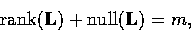
where null(L) represents the dimension of the nullspace of L.
In our case m = 12 and there are three cases to consider:
- rank(L) = 12. Then the nullspace has dimension 0, and there
is only one solution to the system, namely q = 0, which is
not very meaningful.
- rank(L) = 11. Then the nullspace has dimension 1 and there is
a unique solution (up to a scale factor).
- rank(L) < 11. Now there is an infinite number of solutions
to equation (5). One way in which this can happen is if all the reference
points Mi are in a plane.
So to achieve a unique solution to the system (5), we need to ensure that the
reference points Mi are in general position. This means that the
chosen points must not lie in a certain configuration, which can be defined
mathematically but is beyond the scope of this lecture. If six or more
points are chosen at random, and do not lie on a plane, then we can
be confident that this situation will not occur.
It is possible to re-cast the problem of solving equation (5) as a non-linear
minimization problem, where we attempt to minimize the distance
in the image plane between the points mi and the re-projected points
Mi. We can do this by defining the quantity
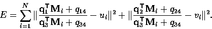
We then use constrained minimization techniques to minimize E, subject
to the constraint that . In general, non-linear methods
lead to much more robust solutions.
Next: References
Up: Computer Vision IT412
Previous: Solving for the calibration
Robyn Owens
10/29/1997