We demonstrate the four classes algorithms described in [14]
on several pairs of frames taken from
sequences of ![]() images.
For the techniques that compare intensity distributions the window size was
images.
For the techniques that compare intensity distributions the window size was
![]() .
The test for the Poisson distribution used
.
The test for the Poisson distribution used ![]() windows.
windows.
![]() was set to 0.01 for the Normal noise intensity model,
while 5% confidence values were used for the test statistics.
Apart from the input images the remaining image are shown inverted to
improve visualisation.
was set to 0.01 for the Normal noise intensity model,
while 5% confidence values were used for the test statistics.
Apart from the input images the remaining image are shown inverted to
improve visualisation.
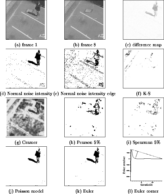
Figures 1a&b show two frames of an outdoor scene containing a pedestrian walking across a carpark. The results of thresholding the difference map (figure 1c) using the Normal model for noise intensity are shown in figure 1d. A reasonable fit using the Normal approximation is made to the difference map histogram, and the walker has been thresholded reasonably well although there is some residual noise. Applying the same technique to a difference image constructed from two frames after running the Sobel edge detector produces a noisier result (figure 1e). In this case the difference map histogram is not so well fit near the tail.
Using the methods for comparing intensity distributions, the Kolmogorov-Smirnov and Cramér-von Mises tests produce the confidence values in figures 1f&g. Both performed poorly in this case since either little or no response is retained after thresholding. We also demonstrate a related approach for comparing two sets of values: correlation. Pearson's rank correlation coefficient is shown thresholded at 0.05 (figure 1h) although the coefficient cannot strictly be interpreted as a probability value. Likewise, a non-parametric method, Spearman's rank correlation, is shown after thresholding in figure 1i. Although the correlation results are better than the distribution comparison results, they are still poor.
Both of the spatial methods (the Poisson noise model and the stable Euler number) produce good results (figures 1j&k). The corner finding procedure is demonstrated on the plot of the Euler number in figure 1l.
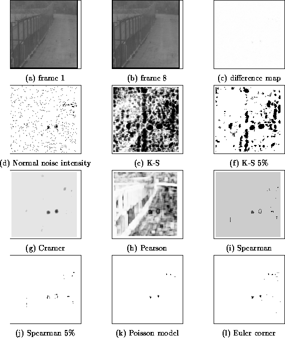
Finally, the images in figures 2a&b are outdoor images from a test surveillance site, taken under a variety of conditions [4], and are rather more demanding. They are poorly illuminated and contain only two sets of small moving objects (rabbits). Due to the low contrast the threshold obtained by the Normal distribution method retains many spurious noise points. The distribution comparison and correlation methods performed poorly (figure 2e-j), either under- or over-thresholding except for Spearman's correlation coefficient which performed quite well. As before, the two spatial methods produced good results (figures 2k&l).
In summary, the two spatial methods (the Poisson noise model and the stable Euler number) generally performed best.

Figure 1: Pedestrian crossing car park

Figure 2: srdb018 image sequence containing moving rabbits