


Next: Texture Boundary
Detection by
Up: Texture Estimation
Previous: texture
represented by histograms.
In the case of non-parametric representation of the texture and by
assuming independent probabilities for the observed pixels (  order Markovian model). For a first order Markov process, the 0th
order statistics of the samples must be an Eigenvector of
order Markovian model). For a first order Markov process, the 0th
order statistics of the samples must be an Eigenvector of  with Eigenvalue
  . Unfortunately, this means that a uniform
prior
for
. Unfortunately, this means that a uniform
prior
for  over is
inconsistent with the uniform prior used in
the 0th order case. To re-establish the consistency, it is necessary
to choose a order prior such that the expected
value of a
column of the transition matrix is
obtained by adding
over is
inconsistent with the uniform prior used in
the 0th order case. To re-establish the consistency, it is necessary
to choose a order prior such that the expected
value of a
column of the transition matrix is
obtained by adding  rather than 1 to the number of observations in that column of the
transition matrix before normalizing the column to sum to . This
means that the transition matrix,
rather than 1 to the number of observations in that column of the
transition matrix before normalizing the column to sum to . This
means that the transition matrix,
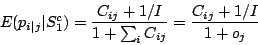 |
(6) |
where  is
the number of times that intensity
is
the number of times that intensity  follows intensity
 in the
sequence
in the
sequence  .
And hence the expected 0th order
distribution
(which is the vector
.
And hence the expected 0th order
distribution
(which is the vector  ) has the
desired
properties since:
) has the
desired
properties since:
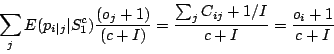 |
(7) |
Which is the
same as Equation 5. This
modification is equivalent to
imposing a prior over
that favors structure
in the Markov
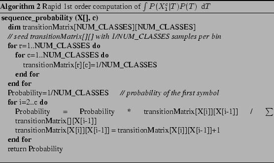
process and is proportional to  ). This
gives Algorithm 2.
). This
gives Algorithm 2.
Next: Texture Boundary
Detection by
Up: Texture Estimation
Previous: texture
represented by histograms.
Ali Shahrokni
2004-06-21