Cartesian moments

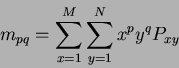
The discrete version of the Cartesian moment (Equation 1.13) for an image consisting of pixels $P_{xy}$, replacing the integrals with summations, is:

$$m_{pq} = \sum_{x=1}^{M} \sum_{y=1}^N x^p y^q P_{xy}$$ (16)

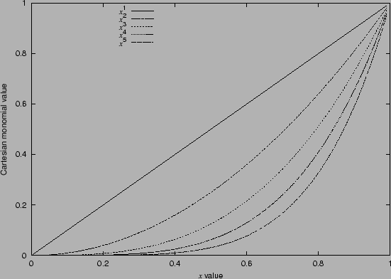
$m_{pq}$Two dimensional Cartesian moment Where $M$ and $N$ are the image dimensions and the monomial product $x^{p}y^{q}$ is the basis function. Figure 1.2 illustrates the non-orthogonal (highly correlated) nature of these monomials (in contrast to the orthogonal polynomials in Figure 1.6, to be discussed later) plotted for the positive $x$ axis only.

Figure 1.2: The first five Cartesian monomials.

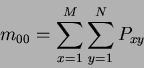
The zero order moment $m_{00}$ is defined as the total mass (or power) of the image. If this is applied to a binary (i.e. a silhouette) $M$$\times$$N$ image of an object, then this is literally a pixel count of the number of pixels comprising the object.

$$m_{00} = \sum_{x=1}^{M} \sum_{y=1}^N P_{xy} %%\mid P_{xy} > 0$$ (17)

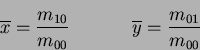
The two first order moments are used to find the Centre Of Mass (COM)COMCentre of mass of an image. If this is applied to a binary image and the results are then normalised with respect to the total mass ($m_{00}$), then the result is the centre co-ordinates of the object. Accordingly, the centre co-ordinates $\overline{x},\overline{y}$$\overline{x}$$x$ axis centre of mass$\overline{y}$$y$ axis centre of mass are given by :

$$\overline{x} = \frac{m_{10}}{m_{00}} ~~~~~~~~~~\overline{y} = \frac{m_{01}}{m_{00}}$$ (18)

The COM describes a unique position within the field of view which can then be used to compute the centralised moments of an image.