This teach file gives an introduction to stereoscopic vision. It also describes perspective projection.
Please read the introduction giving general information about the nature of this document.
You need to have read and understood TEACH VISION1. It will be helpful to have looked at VISION2, VISION3 and VISION4.
This is a long teach file, but it has not been split as the material belongs together. You could split it yourself in two ways. The first is to take it in two parts, perhaps breaking after the section on "Stereo geometry for converging cameras". The second way, which is possibly better, is to go through the file a first time without paying too much attention to the equations and Pop-11 code, but executing the latter so as to see the demonstrations; then on a second pass you could study the equations and look at the code more carefully to see how the ideas are put into practice.
Before proceeding, execute the following chunk of code to avoid having to load the libraries later.
    uses popvision          ;;; search vision libraries
    uses rci_show           ;;; image display
    uses rc_context         ;;; allows multiple windows for graphics
    uses rc_graphplot       ;;; graph drawing
    uses arrayfile          ;;; array storage
    uses float_byte         ;;; type conversion
    uses float_arrayprocs   ;;; array arithmetic
    uses canny              ;;; Canny edge detection
We will need two images of a scene, from different viewpoints, so execute this now:
    vars imageR, imageL;
    arrayfile(popvision_data dir_>< 'stereo1.pic') -> imageR;
    float_byte(imageR, false, false, 0, 255) -> imageR;
    arrayfile(popvision_data dir_>< 'stereo2.pic') -> imageL;
    float_byte(imageL, false, false, 0, 255) -> imageL;
Viewing a scene from two (or more) different positions simultaneously allows us to make inferences about 3-D structure, provided that we can match up corresponding points in the images. The visual systems of humans and some other animals make use of this, and it is very important in attempts to develop practical computer vision systems.
Display the stereo pair of images which we read in above, with:
    1 -> rci_show_scale;        ;;; keep them small
    500 -> rci_show_x;         ;;; set the position for the L window
    350 -> rci_show_y;
    rci_show(imageL) -> ;
    rci_show_x + 120 -> rci_show_x;  ;;; position for the R window
    rci_show(imageR) -> ;
(This code carefully positions the windows beside one another. If you want to move the windows, do it by changing the values for rci_show_x and rci_show_y and re-executing the code, to keep the relative positions the same. Remember that you can get rid of unwanted image windows just by clicking on the image.)
You may find it possible to fuse these images in your own visual system. I did it by iconifying all the other windows so that only the stereo pair was visible against a plain background. (If you have a patterned X background enlarge an xterm or other window to cover most of the screen, and put it behind the images by selecting "back" from its titlebar menu.) I then looked at the images from a distance of about 10 inches (25 cm). So that I could only see the left image with my left eye and the right image with my right eye, I held a piece of A4 card up so that one long edge was against the screen between the two images, and the opposite edge was touching my nose. I consciously relaxed my eyes as if I was looking at something in the distance; although this made the images go out of focus, after a while I could get them to fuse as if I was looking at a single picture. I found I could then get this back into focus without breaking the fusion. At that point it looked as if there was a tiny tripod clearly standing out in front of the screen, with the door handle and other objects in the background further away.
In fact, the Victorians invented technology for presenting stereo pairs more conveniently than this, and were enthusiastic about viewing them. You can still find Victorian stereoscopes and collections of stereo pairs in antique shops. Every so often, film-makers discover they can use stereoscopic presentation to dramatic effect, though the audience has to wear glasses with coloured or polarising filters to ensure that a different image goes to each eye. Map-makers use stereo presentation of aerial photographs to estimate ground topography.
The stereo pair of images on the screen was obtained using two camera positions separated horizontally. Viewing the images normally, you can see how the change in camera position has resulted in a change in the position of the tripod's image relative to the images of other objects. There are two computational issues to address: first, how these image differences can be translated into 3-D information; and second, how the images can be matched to one another so that the differences between them can be measured.
Before we can look at stereo geometry, we need to introduce the relationship between image and object positions for a single camera.
Positions in the image will be expressed using a coordinate system with its origin at the centre of the image, x running from left to right, and y running from bottom to top:
          -----------------------------------------------
          |                      ^                      |
          |               y-axis |                      |
          |                      |                      |
          |                      |                      |
          |                      |                      |
          |                      |                      |
          |                      |                      |
          |                      |                      |
          |  --------------------+------------------->  |
          |                      |             x-axis   |
          |                      |                      |
          |                      |                      |
          |                      |                      |
          |                      |                      |
          |                      |                      |
          |                      |                      |
          |                                             |
          -----------------------------------------------
It is easy to convert from x and y to column and row indices in the array representing the image. If the image centre is at column c0 and row r0, then column = x + c0 and row = r0 - y.
Positions in space will be expressed using 3-D coordinates X, Y and Z (not to be confused with the X and Y used in some earlier files as synonyms for column and row). The (X, Y, Z) system has its origin at the camera lens, with Z pointing out along the optic axis of the camera (i.e. at right angles to the image plane), X parallel to x, and Y parallel to y.
Suppose we have a situation where Y is actually vertical - as is the case for the tripod test images. Then looking down on the camera and scene from above gives this layout of the X and Z coordinate axes :
                                 ^
                          Z-axis |
                                 |
                                 |
                     Objects being viewed in this
                             general area
                                 |
                                 |
                                 |
                                 |
                                 |
                                 |
                           lens ---
                               -- -- ------------------>
                               |   |             X-axis
                       Camera  |   |
                               -----
The Y axis is pointing at you out of the screen. The intersection of the axes is at the optical centre of the camera lens. The (X, Y, Z) system is called camera coordinates because it is fixed with respect to the camera, centred on it, and aligned with it. In robotics, other coordinate systems fixed with respect to an object being manipulated, part of a robot arm, or some mechanical framework in which the robot is working, are often employed as well.
What is the relationship between the camera coordinates of a point in space and the coordinates of its image? If we assume a camera with a planar image surface and no lens distortions (and this camera model is usually quite close to reality), the mathematical form of the relation is quite simple:
                   X f
            x   =  ---
                    Z

                   Y f
            y   =  ---
                    Z
These are the equations of perspective projection. The constant f is the focal length of the camera, and is the distance from the optical centre of the lens to the image plane. X, Y and Z specify the position of a point in space; x and y specify the position of its image in the image plane. These equations allow us to work out x and y if we know X, Y and Z, but do not allow us to go in the other direction, because knowing x and y is not sufficient on its own to pin down the position of the point in 3-D.
There is a simple geometrical derivation of these formulae. A lens behaves approximately like the pinhole of a pinhole camera (except it produces a much brighter image), and so we can draw a straight line from a point in space, through the lens centre, to its image. For a point on the same horizontal level as the camera (Y = 0), the resulting diagram, looking down on the scene as in the diagram above, is:
                                 ^
                          Z-axis |
                                 |         . <- Position of point
                                 |        /|    in space
                                 |       / |
                                 |      /  |
                                 |     /   |
                                 |    /   Z|
                                 |   /     |
                                 |  /      |
                                 | /       |
                    Camera lens  |/   X    |
                    centre ->  --+--------------------->
                                /|                 X-axis
                               / |f
          Position of image \ /  |
          of point          ---------- <- Image plane in camera
                               x
The relation between x and X now follows from similar triangles (via x/f = X/Z). Since a movement along the Y axis will not affect x, this relation continues to hold even if Y is non-zero. The corresponding relation between y and Y is obtained by drawing the side-view diagram.
It looks from the diagram above as if the x-axis has to run from right to left, in the opposite direction to the X-axis. However, if you look at the image actually formed in the camera it is left-to-right inverted and upside-down compared with the way we display the digitised image on the screen. (You can see this with an ordinary camera by putting tracing paper where the film should go, and keeping the back and the lens open.) When we display the image "right way round" on the screen, the x and y axes get flipped, so that they run in the same directions as the X and Y axes. The easiest way to deal with this is to imagine that the camera forms a virtual image which is in front of the lens instead of behind it, and to pretend that this is what gets digitised. The diagram then looks like this:
                                 ^
                          Z-axis |
                                 |         . <- Position of point
                                 |        /     in space
                                 |       /
                                 |      /
                                 |     /
                                 |    /
  Virtual image plane  -> -------+---+---->
                                 |  /   x-axis
                                f| /
                    Camera lens  |/
                    centre ->  --+--------------------->
                                                     X-axis
This is just a different way of modelling the camera; it is less like the reality in terms of physical layout, but it is easier to work with than the image-behind-the-lens model because the virtual image is "right way round". The similar triangles argument still applies, and gives the same mathematical relationships between x and X, and y and Y, so the models are formally equivalent.
The projection equations obviously work if all the quantities are measured in the same units. However, we would normally like to measure distances in the image in pixel units, where 1 pixel unit is just the distance between the centres of two neighbouring pixels, because then array indices correspond to position. Distances in the scene will usually be measured in something like inches or millimetres. It turns out that the x equation is still valid as long as x and f are in the same units as one another, and X and Z are in the same units as one another (and similarly for the y equation). Thus if we know f in pixel units, everything works out conveniently. Finding the value of f in pixel units is basic camera calibration, and is usually best done by making measurements of the image of an object of known size and distance. It is also possible to estimate f in pixel units from the focal length of the lens (usually stamped on it in millimetres) and the number of pixels per millimetre in the camera detector.
Very high accuracy requires a camera model which takes into account lens distortions and detector irregularities. Such models require more elaborate calibration.
Now suppose we have two cameras imaging the scene. It will be simplest to start by assuming that their optical axes are lined up parallel to one another. We also assume that they are side by side - or more exactly, that the line joining their optical centres is parallel to their x-axes. This means that the image of a point will have the same y coordinate for the two cameras. The top view is something like:
                        Objects being viewed

                       in this general region


                        ---                ---
                       -- --              -- --
               Left    |   |      Right   |   |
               Camera  |   |      Camera  |   |
                       -----              -----
Positions in space could be described in either of the two camera coordinate systems, but it is convenient to describe positions relative to an imaginary third camera half-way between the two real cameras. We can call this the cyclopean coordinate system (the cyclops only had one eye in the middle of its head). Schematically, looking down on the scene:
                           ^
                    Z-axis |
                           |
                           |
                           |
              Objects out here specified
                using (X, Y, Z) coords
                           |
                           |
                           |
                           |
                           |
 Left                      |   Right
 image -----+----->        |   image -----+----->
                 xL        |                   xR
                           |
                           |
    --------+--------------+--------------+--------------->
           /                \              \            X-axis
        Left camera          \              \
        optical centre        \              Right camera optical
                               \             centre
                                \
                                 Origin of cyclopean coordinates

            <------------- D ------------->
Here xL and xR are the x coordinates for an image point in the left and right images respectively. D is the separation between the cameras' centres.
Now if a point at (X, Y, Z) in cyclopean coordinates produces images at (xL, y) and (xR, y) in the two cameras, we can find its position in space from the image positions using the formulae:
                          D (xL + xR)
                    X  =  -----------
                          2 (xL - xR)

                            D y
                    Y  =  -------
                          xL - xR

                            D f
                    Z  =  -------
                          xL - xR
The quantity xL-xR which appears in all three formulae is called the stereo disparity (or just the disparity) of the point. It is the difference in the horizontal positions of the images of a point.
D must be measured in the same units as X, Y and Z, and xL, xR, y and f can all be in pixel units.
Deriving these equations is fairly straightforward. The main thing to use is that the perspective projection equations in x for the left and right cameras become xL = (X + D/2)f/Z and xR = (X - D/2)f/Z. This is because to get from X in cyclopean coordinates to X in left or right camera coordinates you simply adjust for the offsets of the cameras from the cyclopean origin, whilst Z is the same in all three coordinate systems. A little algebra then gives the expressions above for X and Z, and that for Y follows easily.
Note the structure of the Z equation. Z is often termed the depth of an object relative to the cameras. A small disparity yields a large depth, and vice versa.
It is not usually convenient to set up the cameras with their axes parallel, because this limits the region of space in which objects are visible in both images. It is more normal to aim the cameras so that their axes are angled inwards, and converge on the objects of interest. The point in space where the optical axes intersect might be described as the fixation point for the cameras. The image of an object at the fixation point is centred for both cameras, and so has zero disparity.
         ^                      . <- Fixation point
         |                     / \
         |                    /   \
         |                   /     \
         |                  /       \
         |                 /         \
         Z0               /     ^     \   <-- Optic axes of cameras
         |               /     Z|      \
         |              /       |       \
         |             /        |        \
         |            /         |         \
         |           /          |          \
         |          /           |           \
         V         O       -----+----->      O
                 Left                X      Right
                 Camera                     Camera
It turns out that this makes the geometry considerably more complicated, and the exact equations for getting from image points to space points are much less straightforward than for parallel cameras. Matching points will not even generally lie at the same y coordinate. Provided the amount of convergence is small, though, we can ignore this vertical disparity, and there is a reasonable approximation which can be used for the equations. Call the depth of the fixation point Z0. Then the disparities can be adjusted by adding the quantity fD/Z0, which is the disparity an object at the fixation point would have if the axes were parallel. The new equations become:
                          D (xL + xR)
                    X  =  -----------
                              2 p

                          D y
                    Y  =  ---
                           p

                          D f
                    Z  =  ---
                           p
                                    f  D
    where           p  =  xL - xR + ----
                                     Z0
Z0 is another parameter that must be found by calibration.
It will be convenient to have the formulae available as a Pop-11 procedure, which we define next.
    define images_to_world(colL, colR, row, c0, r0, D, f, p0)
            -> (X, Y, Z);
        ;;; Calculates the cyclopean coordinates of a point, using
        ;;; the near-parallel approximation. Arguments are:
        ;;;     cL - the column in the left image
        ;;;     cR - the column in the right image
        ;;;     row - the row, assumed same for both images
        ;;;     c0 - the column at the origin of image coords
        ;;;     r0 - the row at the origin of image coords
        ;;;     D - the camera separation in world units
        ;;;     f - the focal length in pixel units
        ;;;     p0 - the disparity shift in pixel units.
        lvars colL, colR, row, c0, r0, D, f, p0, X, Y, Z;
        ;;; Convert from col/row to image coords
        lvars xL, xR, y;
        colL - c0 -> xL;
        colR - c0 -> xR;
        r0 - row -> y;
        ;;; Get adjusted disparity
        lvars p;
        xL - xR + p0 -> p;
        ;;; and apply stereo formulae
        D * (xL + xR) / (2 * p) -> X;
        D * y / p -> Y;
        D * f / p -> Z
    enddefine;
This procedure implements our simplified model of stereo geometry.
(This section and the following one incorporate a fair amount of Pop-11 code. This is to make it easy for you to see what is being done at the programming level, if you want to, and to experiment. However, as pointed out at the start of the file, you can follow the main points simply by executing the Pop-11 sections when you get to them, and reading the text between - you can always return to look at the programs later.)
We are now in a position to work out some of the layout of the tripod stereo pair. We will assume the following parameters for the camera set-up:
    vars
        c0 = 128,    ;;; Column at x-origin, c0   =  128
        r0 = 128,    ;;; Row at y-origin, r0      =  128
        D  =  20,    ;;; Separation, D            =   20 cm
        f  = 200,    ;;; Focal length, f          =  200 pixel units
        Z0 = 100;    ;;; Fixation distance, Z0    =  100 cm
We can define a procedure that converts from image positions to cyclopean coordinates for this specific set-up by making a closure (see HELP *CLOSURES) of our general procedure. We do this with:
    define im_to_w =
            images_to_world(% c0, r0, D, f, D*f/Z0 %)
    enddefine;
Now we need to get some matching points. We will take the edges from the Canny edge detector (see TEACH VISION3) as the features to match, so first apply the Canny operation, and threshold the results to give binary edge maps:
    vars cannL, cannR;
    vars sigma = 1, t1 = 5, t2 = 10;    ;;; Canny parameters
    canny(imageL, sigma, t1, t2) -> ( , , cannL);
    float_threshold(0, t1/2, 1, cannL, cannL) -> cannL; ;;; threshold
    canny(imageR, sigma, t2, t2) -> ( , , cannR);
    float_threshold(0, t1/2, 1, cannR, cannR) -> cannR; ;;; threshold
Display the edge maps with:
    2 -> rci_show_scale;                    ;;; bigger is easier to see
    vars winCL, winCR;                      ;;; to save the windows
    500 -> rci_show_x;                     ;;; position the windows
    rci_show_y + 170 -> rci_show_y;
    rci_show(cannL) -> winCL;
    rci_show_x + 240 -> rci_show_x;
    rci_show(cannR) -> winCR;
(Output is displayed a little further on.)
We need a procedure for getting the features in a given row. This is simple enough:
    define features(image, cstart, cend, row) -> list;
        ;;; Returns a list of the column numbers for which there are
        ;;; non-zero pixels in the given row of the image, between
        ;;; columns cstart and cend.
        lvars image, cstart, cend, row, list;
        lvars col;
        [%                  ;;; start building list
            for col from cstart to cend do
                if image(col, row) /= 0 then
                    col                 ;;; put this column in the list
                endif
            endfor
        %] -> list
    enddefine;
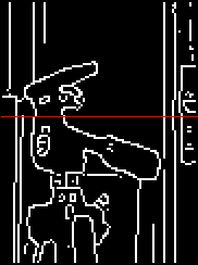
Now we choose a row - say 120, which goes through the tripod head. We'll display the position of this row on the screen:
    vars row = 120;         ;;; set up the row
    winCL -> rc_window;     ;;; draw on the left edge map
    rci_show_setcoords(cannL);  ;;; set the scales correctly
    XpwSetColor(rc_window, 'red') -> ;
    rc_jumpto(83, row);     ;;; draw a line along one row
    rc_drawto(173, row);
    winCR -> rc_window;     ;;; draw on the right edge map
    XpwSetColor(rc_window, 'red') -> ;
    rc_jumpto(83, row);
    rc_drawto(173, row);
and collect the right and left features for it, for all columns from 83 to 173 (i.e. the whole width of the image):
    vars featuresL, featuresR;
    features(cannL, 83, 173, row) -> featuresL;
    features(cannR, 83, 173, row) -> featuresR;
    featuresL ==>
prints:
    ** [100 120 133 159 163 167]
    featuresR ==>
prints:
    ** [90 93 99 112 158 162 166]
The list for the right image has one more entry than that for the left image. Inspecting the edge maps shows that this is due to the fact that the second edge from the left, at column 93 in the right image, is not represented in the left image. We can therefore make the two lists correspond by omitting this feature - of course, this is cheating, and a real stereo system will have to do this automatically. For now, though, do:
    vars reduced_featuresR;
    delete(93, featuresR) -> reduced_featuresR;
Now we can look at what layout the stereo procedure gives. We need a diagram looking down on the tripod - this will produce it, showing the cyclopean coordinate system:
    false -> rc_window; ;;; avoid destroying present rc_window
    rc_new_window(200, 600, 10, 10, false); ;;; start a new window
    [-20 20 0 120] -> rcg_usr_reg;           ;;; set the axis limits
    rc_graphplot([], 'X', [], 'Z') -> ;
Move the window with the mouse if it is not in a convenient place. We can mark the positions of the two cameras, remembering that their separation is D, so they are D/2 either side of the origin:
    XpwSetColor(rc_window, 'red') -> ;
    rcg_plt_square(-D/2, 0);                ;;; mark X = -D/2, Z = 0
    rcg_plt_square( D/2, 0);
Now we can apply our stereo procedure to each pair of features, and plot the corresponding positions in the X-Z plane:
    vars colL, colR, X, Y, Z;
    for colL, colR in featuresL, reduced_featuresR do
        im_to_w(colL, colR, row) -> (X, Y, Z);
        rcg_plt_cross(X, Z)
    endfor;
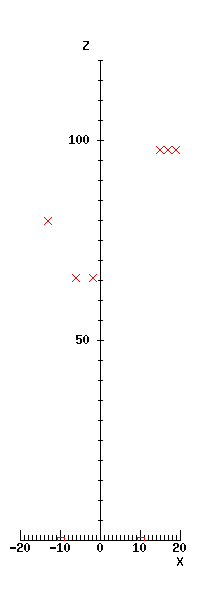
We see the position of the two sides of the tripod head shown at about Z = 66, the object at the left further away at about Z = 80, and three points on the door frame to the right at about Z = 98.
You can easily repeat this with other rows from the image, but it is tedious manually deciding which features to delete in order to make the others match up.
The problem of pairing up the features is known as the correspondence problem. If we apply no constraints, any feature in the left image could match any feature in the right image. A small modification of the code above allows you to display the positions of all the possible matches between the two lists of features.
We have already used the most basic constraint, when we looked for matching features in a single row of the image. That is, we have assumed that a feature with a particular y value can only match a feature in the other image with the same y value. This is known as the epipolar constraint. For converging cameras, using the same y value is actually an approximation, and to be exact we should search for matching features on epipolar lines, which are curves close to the rows of the image. We will continue to use the approximation that the epipolar lines are the same as the image rows.
There remains the problem of matches between all the features with the same y. There are three main constraints that can help:
The bases of these constraints are discussed in various books - those by Frisby and Marr (see TEACH *VISION) are probably best. The first constraint is straightforward to apply, but there is considerable flexibility in the way the other two can be used. We will initially explore the use of the second constraint.
There are many ways of measuring feature similarity. For example, some systems make use of the orientation of the edge. Here we will adopt a measure based on the grey-levels in the image: we will add up the differences in grey-levels in a patch of pixels round the feature, on the assumption that matching regions should have a similar local structure and overall grey-level. To avoid negative and positive differences cancelling out, we will square each difference before doing the addition. Measures like this, based on sums of squares, are extremely common. Since our features are likely to correspond to the boundaries of objects, we will look at two patches, one on each side of the feature, and accept a match if either the grey-level differences to the left of the feature are small, or the differences to the right of the feature are small. (Horizontal edges are no good for matching anyway, so taking left-right patches is reasonable, though one could undoubtedly improve on this using edge orientation information.)
This is implemented in the following procedure:
    define mismatch(col1, col2, row, image1, image2) -> result;
        ;;; Returns a measure of the mismatch between a feature at
        ;;; (col1, row) in image1 and a feature at (col2, row) in
        ;;; image2.
        lvars col1, col2, row, image1, image2, q;
        ;;; These constants set the size of the patches at 5x5
        lconstant rsize = 2, csize = 5;
        lvars r, c, d1, d2, s1=0, s2=0;     ;;; initialise sums
        for r from row-rsize to row+rsize do
            for c from 1 to csize do
                ;;; Get-grey-level differences to left and right
                image1(col1-c, r) - image2(col2-c, r) -> d1;
                image1(col1+c, r) - image2(col2+c, r) -> d2;
                ;;; Add up sums of squares.
                s1 + d1 * d1 -> s1;
                s2 + d2 * d2 -> s2;
            endfor
        endfor;
        min(s1, s2) -> result       ;;; take the smaller mismatch
    enddefine;
The procedure is called mismatch because the larger the result it returns, the worse the match between the two features. To keep the argument lists short, mismatch has the parameters controlling the patch size (5 x 5) built into it. These values happen to be OK for this demonstration, but of course a more general library routine might well have them as arguments.
For a given feature in the left image, we can now pick the feature in the right image which matches it best. We can also do the same thing in reverse, starting from a feature in the right image and looking for the best match in the left image. If the two agree (i.e. two features select each other as closest matches), then it is reasonable to accept the pairing as a definite match. The following procedures implement this. Any feature that is only visible in one image should be weeded out. The first constraint (only one match for any given feature) is built in. In addition, to avoid having to check for wild matches, a disparity limit of 40 pixels is rather arbitrarily built in too - this would, of course, be unacceptable in a library procedure.
    define bestmatch(col1, f2, row, image1, image2) -> b;
        ;;; Returns the best match for the feature at (col1, row) in
        ;;; image1 from the list of features at (col2, row) in image2
        ;;; where col2 is an element of f2.
        ;;; Ignores features with a disparity greater than this limit.
        lconstant disp_limit = 40;
        lvars col1, f2, row, image1, image2, b;
        lvars col2, q, best = false;
        for col2 in f2 do
            if abs(col1 - col2) <= disp_limit then
                mismatch(col1, col2, row, image1, image2) -> q;
                if not(best) or q < best then
                    q -> best;
                    col2 -> b
                endif
            endif
        endfor
    enddefine;

    define findmatches(fL, fR, row, imageL, imageR) -> (newfL, newfR);
        ;;; Given a list of features fL in the left image and fR in the
        ;;; right image, returns two lists of the same length which
        ;;; contain features in one-to-one correspondence.
        lvars fL, fR, row, imageL, imageR, newfL = [], newfR = [];
        lvars colL, colR;
        for colL in fL do
            ;;; Find best match for left feature
            bestmatch(colL, fR, row, imageL, imageR) -> colR;
            ;;; Find best match for right feature, and see if it agrees
            if colR     ;;; test there is some matching feature
            and bestmatch(colR, fL, row, imageR, imageL) == colL then
                colL :: newfL -> newfL;
                colR :: newfR -> newfR
            endif
        endfor;
        ;;; Make the lists run left to right (not essential)
        ncrev(newfL) -> newfL;
        ncrev(newfR) -> newfR
    enddefine;
That then provides the basis of a simple stereo matching program, using grey-level matching starting from edge features. Applied to the features we had before, it gives:
    findmatches(featuresL, featuresR, row, imageL, imageR)
        -> (featuresL, featuresR);
    featuresL =>
prints:
    ** [100 120 133 159 163 167]
    featuresR =>
prints:
    ** [90 99 112 158 162 166]
- the feature at column 93 in the right image has been omitted, as required for a correct set of matches.
We can check how this behaves on the complete images. We need a procedure to iterate over rows and get all the matches. We will store each match as a vector containing the column and row numbers, and place all of them in one long vector.
    define findallmatches(imageL, imageR, edgeL, edgeR) -> matchvec;
        ;;; Returns the columns and row for each pair of matching
        ;;; features in the two images. edgeL and edgeR must be the edge
        ;;; maps for imageL and imageR.
        lvars imageL, imageR, edgeL, edgeR, matchvec;
        lvars row, featuresL, featuresR, colL, colR,
            (ic0, ic1, ir0, ir1) = explode(boundslist(imageL)),
            (ec0, ec1, er0, er1) = explode(boundslist(edgeL));
        ;;; Must avoid pixels adjacent to the boundaries to ensure
        ;;; matching procedure does not try to go outside the array.
        ;;; Next constants must correspond to those in mismatch
        lconstant rsize = 2, csize = 5;
        lvars
            cstart = max(ec0, ic0 + csize),
            cend = min(ec1, ic1 - csize);
        {%      ;;; start building big vector
            for row from max(er0, ir0+rsize) to min(er1, ir1-rsize) do
                ;;; Get the features.
                features(edgeL, cstart, cend, row) -> featuresL;
                features(edgeR, cstart, cend, row) -> featuresR;
                ;;; Find one-to-one matches
                findmatches(featuresL, featuresR, row, imageL, imageR)
                    -> (featuresL, featuresR);
                ;;; Get the matches for this row into vectors
                for colL, colR in featuresL, featuresR do
                    {% colL, colR, row %}  ;;; left on stack
                endfor
            endfor
            %} -> matchvec;     ;;; finish building big vector
    enddefine;
This involves a fair amount of computation, so the next step will take some time:
    vars matchvec;
    findallmatches(imageL, imageR, cannL, cannR) -> matchvec;
(The program could be made more efficient, since it calculates many match strengths twice.)
We now have all the matches. First, we can use them to plot all the matches in the (Z, Y) plane, superimposing different X values. This gives a side view of the scene, with the camera positions both at the origin. The cameras are looking left to right in the diagram drawn by the code that follows.
    rc_new_window(300, 300, rci_show_x, rci_show_y, false);
    [0 120 -60 60] -> rcg_usr_reg;      ;;; set coord region
    rc_graphplot([], 'Z', [], 'Y') -> ; ;;; show coords, set scales
    XpwSetColor(rc_window, 'red') -> ;

    appdata(matchvec,
        procedure(match);
            lvars match, X, Y, Z;
            ;;; Use the 2-D to 3-D procedure.
            im_to_w(explode(match)) -> (X, Y, Z);
            rc_drawpoint(Z, Y);
        endprocedure);
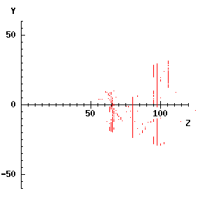
The results are far from perfect, but the tripod at about Z = 65, the object at the left at Z = 80, and the background objects at Z = 90 to 110 show up clearly, with a few false matches scattered around. The results can also be projected onto the (X, Z) plane, which you can try, or indeed plotted as if they were viewed from any given direction, though that requires coordinate rotations which cannot be covered here.
Second, we can look at the matches superimposed on the edge maps, by colour-coding the features according to disparity.
    vars colours = {'red' 'blue' 'green' 'yellow' 'purple' 'orange'
        'pink' 'firebrick' 'magenta' 'brown'};
    rci_show_setcoords(cannL);  ;;; Set coord system
    appdata(matchvec,
        procedure(match);
            lvars match, colL, colR, row, colour;
            dlocal rc_window;
            explode(match) -> (colL, colR, row);
            ;;; arbitrary mapping from disparities to colours
            colours((colL-colR+40) div 8 + 1) -> colour;
            winCL -> rc_window;
            XpwSetColor(rc_window, colour) -> ;
            rci_drawpoint(colL, row);
            winCR -> rc_window;
            XpwSetColor(rc_window, colour) -> ;
            rci_drawpoint(colR, row);
        endprocedure);
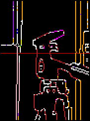
This makes it easy to see where incorrect matches have occurred, and also provides a form of depth map of the scene, with different colours indicating different distances away from the camera.
Although matching based on grey-level least-squares differences worked reasonably well, it is computationally quite expensive, and there were some erroneous matches. One way round these problems might be to match higher-level features, such as straight line segments, and this kind of approach is sometimes used in practice.
Another set of techniques involves using the third constraint listed above: that points near each other in the image will usually have similar disparities, because the scene is made of coherent surfaces This constraint has been formalised in various ways, for example in terms of the disparity gradient limit used in the system developed by a group at Sheffield, described in detail in TEACH *PMF. Prior to that, the constraint was discussed by Marr and used in an interesting way in his cooperative algorithm for finding correspondences. Using disparity smoothness is probably particularly appropriate when trying to match images with a high density of features, as is the case with random dot stereograms. It would be less suitable for the rather sparse features we have been working with.
Marr also proposed a method of stereo matching based on scale space ideas. In this, the zero-crossings of large-scale DoG filters are matched initially, giving rough estimates for the disparities; these are used as a guide to initial disparities for matching at a smaller scale, and so on until matching is done on the smallest visible details at high accuracy. Nishihara developed this approach in a program intended for real-time stereo matching, which works on the kind of binary images displayed in the zero-crossing section of TEACH VISION3.
A rather different way of estimating stereo disparities has recently become prominent. In this, the outputs of a set of convolution masks, sensitive to particular spatial frequencies (see TEACH VISION3), are used to estimate local phase shifts between the left and right images. This kind of method is probably best suited to images with small disparities.
On a first reading, you should:
When you have followed the file in detail, you should also:
Here are links to:
Copyright University of Sussex 1994. All rights reserved.