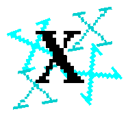


Like other image arithmetic operators, multiplication comes in two main forms. The first form takes two input images and produces an output image in which the pixel values are just those of the first image, multiplied by the values of the corresponding values in the second image. The second form takes a single input image and produces output in which each pixel value is multiplied by a specified constant. This latter form is probably the more widely used and is generally called scaling.
This graylevel scaling should not be confused with geometric scaling.
The multiplication of two images is performed in the obvious way in a single pass using the formula:
Scaling by a constant is performed using:
Note that the constant is often a floating point number, and may be less than one, which will reduce the image intensities. It may even be negative if the image format supports that.
If the pixel values are actually vectors rather than scalar values (e.g. for color images) then the individual components (e.g. ref{rgb}{red, blue and green components}) are simply multiplied separately to produce the output value.
If the output values are calculated to be larger than the maximum allowed pixel value, then they may either be truncated at that maximum value, or they can `wrap around' and continue upwards from the minimum allowed number again.
There are many specialist uses for scaling. In general though, given a scaling factor greater than one, scaling will brighten an image. Given a factor less than one, it will darken the image. Scaling generally produces a much more natural brightening/darkening effect than simply adding an offset to the pixels, since it preserves the relative contrast of the image better. For instance,
shows a picture of model robot that was taken under low lighting conditions. Simply scaling every pixel by a factor of 3, we obtain
which is much clearer. However, when using pixel multiplication, we should make sure that the calculated pixel values don't exceed the maximum possible value. If we, for example, scale the above image by a factor of 5 using a 8-bit representation, we obtain
All the pixels which, in the original image, have a value greater than 51 exceed the maximum value and are (in this implementation) wrapped around from 255 back to 0.
The last example shows that it is important to be aware of what will happen if the multiplications result in pixel values outside the range that can be represented by the image format being used. It is also very easy to generate very large numbers with pixel-by-pixel multiplication. If the image processing software supports it, it is often safest to change to an image format with a large range, e.g. floating point, before attempting this sort of calculation.
Scaling is also often useful prior to other image arithmetic in order to prevent pixel values going out of range, or to prevent integer quantization ruining the results (as in integer image division).
Pixel-by-pixel multiplication is generally less useful, although sometimes a binary image can be used to multiply another image in order to act as a mask. The idea is to multiply by 1 those pixels that are to be preserved, and multiply by zero those that are not. However for integer format images it is often easier and faster to use the logical operator AND instead.
Another use for pixel by pixel multiplication is to filter images in the frequency domain. We illustrate the idea using the example of
First, we obtain
by applying the Fourier transform to the original image, and then we use pixel multiplication to attenuate certain frequencies in the Fourier domain. In this example we use a simple lowpass filter which (as a scaled version) can be seen in
The result of the multiplication is shown in
Finally, an inverse Fourier transform is performed to return to the spatial domain. The final result
shows the smoothing effect of a lowpass filter. More details and examples are given in the worksheets dealing with frequency filtering.
You can interactively experiment with this operator by clicking here.
and its skeleton
using pixel addition (the skeleton was derived from
which was produced by thresholding the input image at 110). Use image multiplication to scale the images prior to the addition in order to avoid the pixel values being out of range. What effect does this have on the contrast of the input images.
into foreground and background. Use scaling to set the foreground pixel value to 2, and the background pixel value to 0. Then use pixel-by-pixel multiplication to multiply this image with the original image. What has this process achieved and why might it be useful?
E. Davies Machine Vision: Theory, Algorithms and Practicalities, Academic Press, 1990, Chap. 2.
A. Marion An Introduction to Image Processing, Chapman and Hall, 1991, p 244.
Specific information about this operator may be found here.
More general advice about the local HIPR installation is available in the Local Information introductory section.


