Additional SURFACE Feature Location

Given the initial location estimates and the geometric model, it is easy to predict where a visible surface should appear. This prediction simplifies direct search for image evidence for the feature. This is, in style, like the work of Freuder [75], except that three dimensional scenes are considered here.

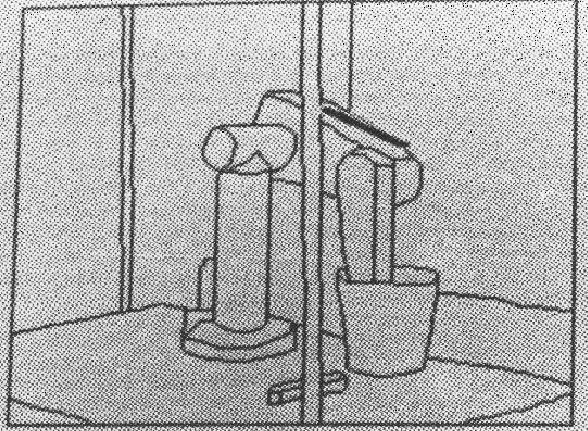
To select good image evidence for an uninstantiated model feature, the oriented model is used to predict roughly where the surface data should appear. Figure 9.20 shows the predicted location for the robot upper arm $uedgel$ panel superimposed on the original image using the initial parameter estimates for $upperarm$.

Figure 9.20: Predicted Uedgel Panel on Image

Other constraints can then be applied to eliminate most inappropriate surfaces from the predicted area. The constraints that a potential surface must meet are:

1. It must not be previously used.
2. It must be in the surface cluster for the ASSEMBLY.
3. It must be in the correct image location.
4. It must have the correct three dimensional surface orientation.
5. It must have the correct three dimensional location.
6. It must have the correct size.
7. Its visible portions must have the correct shape.

The implemented algorithm used the constraints 1 to 5, with some parameter tolerances on 3, 4 and 5. The $7^{th}$ was not used because likely causes for not finding the surface during invocation were: it was partially obscured, it was incompletely segmented or it was merged during the surface reconstruction process (Chapter 4). The result of these would be incorrect shapes. These factors also affect the area constraint (6), so this was used only to select a single surface if more than one met the first five constraints (but this did not occur in the test scene).

The implemented algorithm is:

Let:
	S = {all surfaces in the surface cluster not previously used in the hypothesis} = {$s_d$}
	$\vec{c}_p$ = predicted image central point for the missing SURFACE
	$\vec{c}_d$ = observed image central point for $s_d$
	$\vec{n}_p$ = predicted three dimensional surface normal at $\vec{c}_p$
	$\vec{n}_d$ = observed three dimensional surface normal at $\vec{c}_d$
	$z_p$ = predicted depth at $\vec{c}_p$
	$z_d$ = observed depth at $\vec{c}_d$
	$A_p$ = model area for missing SURFACE
	$A_d$ = estimated area for $s_d$

If:
	(constraint 3)
	$\mid \vec{c}_d - \vec{c}_p \mid < \tau_1$	($\tau_1$ = 20 pixels)
	(constraint 4)
	$\vec{n}_p \circ \vec{n}_d > \tau_2$	($\tau_2$ = 0.8)
	(constraint 5)
	$\mid z_p - z_d \mid < \tau_3$	($\tau_3$ = 50 cm)
Then:	$s_d$ is an acceptable surface

The surface selected is the acceptable $s_d$ whose area is closest to that predicted, by minimizing:

$$\mid 1 - \frac{A_d}{A_p} \mid$$

In the test image, the only missing SURFACEs were the two side surfaces on the upper arm and the inside surface at the back of the trash can. For the trash can, the only potential image surfaces for the trash can back surface were the two visible surfaces in the surface cluster. The front surface was already used in both cases, and the rear surface met all the other constraints, so was selected. A similar process applied to the upper arm side panels.