A local approximation : the osculating paraboloïd

Since ${\cal S}$ is a smooth surface, a neighbourhood of a point P on ${\cal S}$ can be represented in the form z= h(x,y), where P is the origin of the coordinate frame and the z axis is directed by the normal N of ${\cal S}$ at P. Thus the xy plane is the tangent plane to ${\cal S}$ at P. Moreover, h is a differentiable function and by taking Taylor's expansion at P, we have:

$$h(x,y)= z= \frac{1}{2}(h_{xx} x^2+ 2h_{xy} xy+h_{yy}y^2) + R(x,y),$$

where R(x,y) satisfies:

$$\lim_{(x,y) \rightarrow (0,0) } \frac{R(x,y)}{x^2+y^2}=0.$$

The quadratic form $\frac{1}{2}(h_{xx} x^2+ 2h_{xy} xy+h_{yy}y^2)$ is known as the Hessian of h at (0,0) and corresponds to the second fundamental form of ${\cal S}$ at P. The quadratic surface ${\cal Q}$ defined by

$${\cal Q}=\{(x,y,z) ,z = \frac{1}{2}(h_{xx} x^2+ 2h_{xy} xy+h_{yy}y^2)\}$$

approximates ${\cal S}$ up to order 2. This surface is called the osculating paraboloïd of ${\cal S}$ at P and is uniquely defined.

We first assume that the x and y axes are oriented by T and $r_s/\left\vert r_s\right\vert$ respectively, where T is the viewing direction and r_s the tangent to the rim of ${\cal S}$ at P. Since these directions are conjugate [Koe 84], the first and second fundamental forms of ${\cal S}$ at P, in the parametrisation (x,y), are:

$$I_P = \left[ \begin {array}{cc} 1 & \cos\theta \ \cos\the... ...egin {array}{cc} k_t & 0 \ 0 & k_s \ \end {array} \right],$$

where $\theta$ is the angle between T and r_s, k_t is the normal curvature along the viewing direction T, and k_s is the normal curvature of the rim at P. Note that k_t is the normal curvature of the epipolar curve at P. Therefore, the osculating paraboloïd of ${\cal S}$ at P is defined, in the parametrisation (x,y), by:

$${\cal Q}=\{(x,y,z) ,z = \frac{1}{2}(k_t x^2 + k_s y^2)\}.$$ (3)

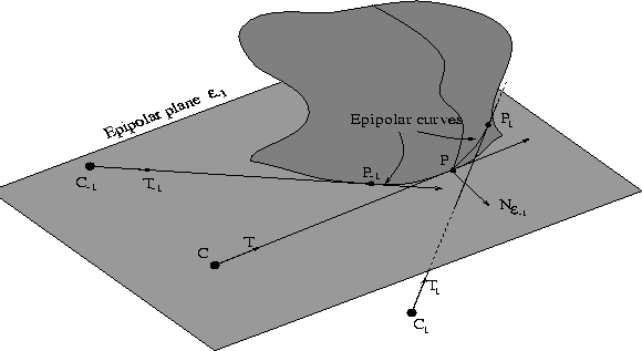
We denote by ${\cal E}_{-1}$ and ${\cal E}_1$ the epipolar planes at a point $P \in {\cal S}$corresponding to three successive positions of the camera centre C_-1, C and C₁, i.e., planes (C,C_-1,P) and (C,C₁,P) (see figure 7). The point P is therefore a point belonging to the rim observed from C. For a general motion ${\cal E}_{-1}$ and ${\cal E}_1$ are different (they are identical for a linear motion). The intersection of one epipolar plane with the surface ${\cal S}$ is a curve. By abuse of language, we call these curves epipolar curves and we have then the following property:

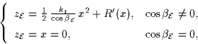
Proposition 2 In any epipolar plane ${\cal E}$ at P, the epipolar curve is, up to the order 2, the graph of the following function:

$$z_{\cal E}= g(x) = \frac{1}{2}\frac{k_t}{\cos \beta_{\cal E}} x^2,$$ (4)

where the x axis is directed by T|_P, the $z_{\cal E}$ axis is such that $(x,z_{\cal E})$ form an orthonormal basis of ${\cal E}$ and $\beta_{\cal E}$ is the angle between the normal N to the surface at P and the projection $N_{\cal E}$ of N in the epipolar plane: $\cos \beta_{\cal E} = N.N_{\cal E}$.

Proof.  Near the point P, we have the following description of ${\cal S}$: 

$$z = \frac{1}{2}(k_t\,x^2 + k_s\,y^2) + R(x,y),$$ (5)

with $\lim_{(x,y) \rightarrow (0,0) } R(x,y)\;/\;(x^2+y^2) = 0.$
Let ${\cal E}$ be an epipolar plane at P and let $\beta_{\cal E}$ be the angle between the normal N to ${\cal S}$ at P and its projection $N_{\cal E}$ in ${\cal E}$. The equation of this plane can be written as:

$$z\, \sin \beta_{\cal E} = y\, \cos\beta_{\cal E} \, \sin\theta,$$

where $\theta$ is the angle between the x axis and the y axis (or equivalently between T and r_s at P). Now if the $z_{\cal E}$ axis is defined such that $(x,z_{\cal E})$ forms an orthonormal basis of ${\cal E}$, we have:

$$z = z_{\cal E} \, cos\beta_{\cal E}.$$

The epipolar curve is the intersection of the plane ${\cal E}$ with the surface ${\cal S}$, therefore by substituting in (6) and neglecting third order and higher terms we obtain for points on these curves:  

$$z_{\cal E}\,\cos\beta_{\cal E} = \frac{1}{2}(k_t\,x^2 + \frac{\sin^2\beta_{\cal E} }{\sin^2\theta}\,k_s\,z_{\cal E}^2),$$ (6)

In general, the term $\frac{\sin^2\beta_{\cal E} }{\sin^2\theta}\,k_s$ in (7) can be considered as bounded since:

1.

the case $\sin \theta = 0$ happens only when P is observed along an asymptotic direction which yields a cusp on the occluding contour.

2.

The curvature k_s, which is linked to the curvature of the occluding contour, is finite in our context (the observed object is smooth).

Thus, solving (7) for $(x,z_{\cal E})$ close to (0,0) yields:

$$\left\{ \begin{array} {ll} z_{\cal E} = \frac{1}{2}\, \frac{... ... z_{\cal E} = x = 0, & \cos\beta_{\cal E}= 0,\end{array}\right.$$

with: $\lim_{x \rightarrow 0 } R'(x)\;/\;x^4 = 0$. This shows that up to second order, the epipolar curve is represented by:

$$z_{\cal E} = \frac{1}{2}\, \frac{k_t}{\cos\beta_{\cal E}} \, x^2, \hspace{2cm} \cos\beta_{\cal E} \neq 0.$$

The case $\cos\beta_{\cal E} = 0$ occurs when P is a multiple point, the epipolar curve is then restricted to a single point P.$\square$

Remark The approximation given in proposition 2 verifies the Meusnier's theorem [dC 76] which says that the curvature at P of the epipolar curve is $k = \frac{k_t}{\cos\beta_{\cal E}}$. However, it should be noticed that a local approximation of the epipolar curve based on a circle verifies also Meusnier's theorem. But such approximation implicitely implies that the surface is locally spherical which is less general than the osculating paraboloïd model.

Note that in the above proposition, the x axis is the one previously defined in the parametrisation (x,y) and is thus independent of the epipolar plane.

Since P is the origin of the x axis, proposition 2 says that the epipolar curve depends on the position of P in the epipolar plane (i.e., its depth) and on the normal curvature k_t of ${\cal S}$ along the viewing direction. Our purpose is to recover the position of a rim point P using three successive occluding contours of ${\cal S}$, therefore this can be done by estimating epipolar curves. In the general case there are two different epipolar planes ${\cal E}_{-1}$ and ${\cal E}_1$ for a point P and three successive camera positions, thus there are also two epipolar curves. Since we can match, in the corresponding images, epipolar correspondents, we know two tangents to each epipolar curve (see figure 7). The following section shows how to compute epipolar curves given these tangents.

  

Figure 7: Epipolar curves.