Assuming the errors have a Gaussian distribution, the inverse Hessian matrix of a chi-square distribution of function parameters, sufficiently close to the minimum, is the estimated covariance matrix of standard errors of these parameters.
If we are close enough to the minimum, ![]() , the
, the ![]() distribution of the parameters can be approximated by a quadratic form (Taylor series expansion):
distribution of the parameters can be approximated by a quadratic form (Taylor series expansion):
![]()
as there is no gradient at the minimum, the second term will disappear.
The gradient of the Chi-square distribution wrt to an element of ![]() is:
is:
![]()
Taking another partial derivative:
![]()
As ![]() is a random measurement error that can have either sign, summing over them will cause the second term will disappear.
is a random measurement error that can have either sign, summing over them will cause the second term will disappear.
Now the Hessian is:
![]()
Once we have the value for H, we can invert it and use it as an estimate of the error covariance of the parameters.
![]()
By using the gradient of each datapoint wrt to each parameter, we can use error propagation (see appendix A) to estimate the errors:
![]()
The diagonal elements of this covariance matrix give the probable error at each datapoint.
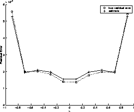
We put this method to the test for fitting a polynomial ![]() with a data measurement accuracy (standard error) of 0.08 on each element. Figure 4 shows a comparison of the predicted error on each datapoint against the true error (averaged over 1000 fits), as found by a least-squares fit. The script error_estimation.m demonstrates this.
with a data measurement accuracy (standard error) of 0.08 on each element. Figure 4 shows a comparison of the predicted error on each datapoint against the true error (averaged over 1000 fits), as found by a least-squares fit. The script error_estimation.m demonstrates this.

Figure 4: Error prediction on ![]() with an error of
with an error of ![]() on each point
on each point