Rectification of camera matrices

We assume that the stereo rig is calibrated, i.e., the PPMs $\tilde{\bf P}_{o 1}$ and $\tilde{\bf P}_{o 2}$ are known. The idea behind rectification is to define two new PPMs $\tilde{\bf P}_{n 1}$and $\tilde{\bf P}_{n 2}$ obtained by rotating the old ones around their optical centers until focal planes becomes coplanar, thereby containing the baseline. This ensures that epipoles are at infinity, hence epipolar lines are parallel. To have horizontal epipolar lines, the baseline must be parallel to the new X axis of both cameras. In addition, to have a proper rectification, conjugate points must have the same vertical coordinate. This is obtained by requiring that the new cameras have the same intrinsic parameters. 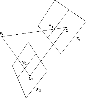Note that, being the focal length the same, retinal planes are coplanar too, as in Figure 2.

  

Figure 2: Rectified cameras. Retinal planes are coplanar and parallel to the baseline.

In summary: positions (i.e, optical centers) of the new PPMs are the same as the old cameras, whereas the new orientation (the same for both cameras) differs from the old ones by suitable rotations; intrinsic parameters are the same for both cameras. Therefore, the two resulting PPMs will differ only in their optical centers, and they can be thought as a single camera translated along the X axis of its reference system.

Let us write the new PPMs in terms of their factorization. From (2) and (7):

$$\tilde{\bf P}_{n1} = {\bf A} [{\bf R}\; \vert- {\bf R} \; {\b... ...bf P}_{n2} = {\bf A} [{\bf R}\; \vert- {\bf R} \; {\bf c}_2] .$$ (9)

The intrinsic parameters matrix ${\bf A}$ is the same for both PPMs, and can be chosen arbitrarily (see MATLAB code). The optical centers ${\bf c}_1$ and ${\bf c}_2$ are given by the old optical centers, computed with (6). The matrix ${\bf R}$, which gives the camera's pose, is the same for both PPMs. It will be specified by means of its row vectors

$${\bf R}= \begin{bmatrix} {\bf r}_1^\top\\ {\bf r}_2^\top\\ {\bf r}_3^\top \end{bmatrix}$$ (10)

that are the X, Y, and Z axes, respectively, of the camera reference frame, expressed in world coordinates.

According to the previous comments, we take:

1.

The new X axis parallel to the baseline: ${\bf r}_1 = ({\bf c}_1 - {\bf c}_2)/\vert\vert {\bf c}_1 - {\bf c}_2 \vert\vert$

2.

The new Y axis orthogonal to X (mandatory) and to ${\bf k}$: ${\bf r}_2 = {\bf k} \wedge{\bf r}_1$

3.

The new Z axis orthogonal to XY (mandatory) : ${\bf r}_3 = {\bf r}_1 \wedge{\bf r}_2$

In point 2, ${\bf k}$ is an arbitrary unit vector, that fixes the position of the new Y axis in the plane orthogonal to X. We take it equal to the Z unit vector of the old left matrix, thereby constraining the new Y axis to be orthogonal to both the new X and the old left Z.

This algorithm fails when the optical axis is parallel to the baseline, i.e., when there is a pure forward motion.