Stratification

Let us assume that a projective reconstruction is available, that is a sequence $\{ \tilde{\bf P}^i_{\mathrm{proj}} \}$ of camera matrices such that:

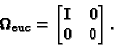
$$\tilde{\bf P}^0_{\mathrm{proj}} = [{\bf I} \;\vert\; {\bf0}] ... ...{\bf P}^i_{\mathrm{proj}} = [{\bf Q}^i \;\vert\; {\bf q}^i] .$$ (24)

We are looking for a Euclidean reconstruction, that is a $4 \times 4$nonsingular matrix $\tilde{\bf T}$ that upgrades the projective reconstruction to Euclidean. If $\{\tilde {\bf w}_j \}$ is the sought Euclidean structure, $\tilde{\bf T}$ must be such that: $\tilde{\bf m}_j^i = \tilde{\bf P}^i_{\mathrm{proj}} \tilde{\bf T} \tilde{\bf T} ^{-1} \tilde{\bf w}_j,$ hence

$$\tilde{\bf P}^i_{\mathrm{eucl}} \simeq\tilde{\bf P}^i_{\mathrm{proj}} \tilde{\bf T} \; ,$$ (25)

where the symbol $\simeq$ means ``equal up to a scale factor.''

Using additional information

Projective reconstruction differs from Euclidean by an unknown projective transformation in the 3-D projective space, which can be seen as a suitable change of basis. Thanks to the fundamental theorem of projective geometry [41], a collineation in space is determined by five points, hence the knowledge of the true (Euclidean) position of five points allows to compute the unknown $4 \times 4$matrix $\tilde{\bf T}$ that transform the Euclidean frame into the projective frame. 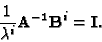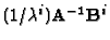Moreover, if intrinsic parameters ${\bf A}$ are known, then $\tilde{\bf T}$ can be computed by solving a linear system of equations (see (54) in Sec. 5.2.5).

Euclidean reconstruction from constant intrinsic parameters

The challenging problem is to recover $\tilde{\bf T}$ without additional information, using only the hypothesis of constant intrinsic parameters. The works by Hartley [17], Pollefeys and Van Gool [37], Heyden and Åström  [20], Triggs [46] and Bougnoux [4] will be reviewed, but first we will make some remarks that are common to most of the methods.

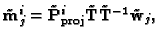
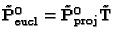
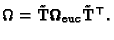
We can choose the first Euclidean-calibrated camera to be $\tilde{\bf P}^0_\mathrm{eucl} = {\bf A} [{\bf I} \;\vert\; {\bf0}]$, thereby fixing arbitrarily the rigid transformation:

$$\tilde{\bf P}^0_{\mathrm{eucl}} = {\bf A} [{\bf I} \;\vert\; ... ...^i_{\mathrm{eucl}} = {\bf A} [{\bf R}^i \;\vert\; {\bf t}^i] .$$ (26)

With this choice, it is easy to see that $\tilde{\bf P}^0_{\mathrm{eucl}} = \tilde{\bf P}^0_{\mathrm{proj}} \tilde{\bf T}$ implies

$$\tilde{\bf T} = \begin{bmatrix} {\bf A}&{\bf0}\\ {\bf r}^\top&s\\ \end{bmatrix}$$ (27)

where ${\bf r}^\top$ is an arbitrary vector of three elements $[r_1 \; r_2 \; r_3]$. Under this parameterization $\tilde{\bf T}$ is clearly non singular, and being defined up to a scale factor, it depends on eight parameters (let s=1).

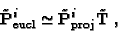
Substituting (24) in (25) one obtains

$$\tilde{\bf P}^i_{\mathrm{eucl}} \simeq\tilde{\bf P}^i_{\mathr... ...bf Q}^i{\bf A} + {\bf q}^i {\bf r}^\top\;\vert\; {\bf q}^i ] ,$$ (28)

and from (26)

$$\tilde{\bf P}^i_{\mathrm{eucl}} = {\bf A} [{\bf R}^i \;\vert\; {\bf t}^i] = [ {\bf A} {\bf R}^i \;\vert\; {\bf A}{\bf t}^i] ,$$ (29)

hence

$${\bf Q}^i {\bf A} + {\bf q}^i {\bf r}^\top\simeq{\bf A} {\bf R}^i .$$ (30)

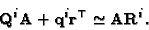
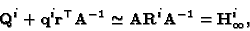
This is the basic equation, relating the unknowns ${\bf A}$ (five parameters) and ${\bf r}$ (three parameters) to the available data ${\bf Q}^i$ and ${\bf q}^i$. ${\bf R}$ is unknown, but must be a rotation matrix.

Affine reconstruction.

Equation (30) can be rewritten as

$${\bf Q}^i + {\bf q}^i {\bf r}^\top{\bf A}^{-1} \simeq{\bf A} {\bf R}^i {\bf A}^{-1} = {\bf H}^i_\infty,$$ (31)

relating the unknown vector ${\bf a}^\top= {\bf r}^\top{\bf A}^{-1}$ to the homography of the infinity plane (compare (31) with (18)). It can be seen that $\tilde{\bf T}$ factorizes as follows

$$\tilde{\bf T} = \begin{bmatrix} {\bf I}&{\bf0}\\ {\bf a}^\t... ...in{bmatrix} {\bf A}&{\bf0}\\ {\bf0}^\top&1\\ \end{bmatrix} .$$ (32)

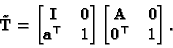
The right-hand matrix is an affine transformation, not moving the infinity plane, whereas the left-hand one is a transformation moving the infinity plane.

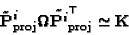
Substituting the latter into (25) we obtain:

$$\tilde{\bf P}^i_{\mathrm{eucl}} \begin{bmatrix} {\bf A}^{-1}... ...&1\\ \end{bmatrix} = [{\bf H}_{\infty}^{i} \vert {\bf q}^{i}]$$ (33)

Therefore, the knowledge of the homography of the infinity plane (given by ${\bf a}$) allows to compute the Euclidean structure up to an affine transformation, that is an affine reconstruction.

From affine to Euclidean.

Another useful observation is, if ${\bf H}_{\infty}$ is known and the intrinsic parameters are constant, the intrinsic parameters matrix ${\bf A}$ can easily be computed [1,17,30,49].

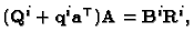
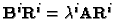
Let us consider the case of two cameras. If ${\bf A}' = {\bf A}$, then ${\bf H}_{\infty}$ is exactly known (with the right scale), since

$$\det({\bf H}_{\infty}) {=} \det ({\bf A}{\bf R}{\bf A}^{-1} ) = 1.$$ (34)

From (17) we obtain ${\bf R} = {\bf A}^{\prime -1}{\bf H}_{\infty} {\bf A},$ and, since ${\bf R}{\bf R}^{\top} = {\bf I}$, it is easy to obtain:

$${\bf H}_{\infty}{\bf K}{\bf H}_{\infty}^{\top} = {\bf K}$$ (35)

where ${\bf K} = {\bf A}{\bf A}^{\top}$ is the Kruppa coefficients matrix. As (35) is an equality between $3\times3$symmetric matrices, we obtain a linear system of six equations in the five unknown k₁, k₂, k₃, k₄, k₅ . In fact, only four equations are independent [30,49], hence at least three views (with constant intrinsic parameters) are required to obtain an over-constrained linear system, which can be easily solved with a linear least-squares technique.

Note that two views would be sufficient under the usual assumption that the image reference frame is orthogonal ( $\gamma = 0$), which gives the additional constraint k₃ k₅ = k₂.

If points at infinity (in practice, sufficiently far from the camera) are in the scene, ${\bf H}_{\infty}$ can be computed from point correspondences, like any ordinary plane homography [49]. Moreover, with additional knowledge, it can be estimated from vanishing points or parallelism [7,9], or constrained motion [1].

In the rest of the section, some of the most promising stratification techniques will be reviewed.

Hartley

Hartley [17] pioneered this kind of approach. Starting from (30), we can write

$$({\bf Q}^i + {\bf q}^i {\bf a}^\top){\bf A} \simeq{\bf A} {\bf R}^i .$$ (36)

By taking the QR decomposition of the left-hand side we obtain an upper triangular matrix ${\bf B}^i$ such that $({\bf Q}^i + {\bf q}^i {\bf a}^\top){\bf A} = {\bf B}^i {\bf R}^i ,$ so (36) rewrites ${\bf B}^i {\bf R}^i = \lambda^i {\bf A} {\bf R}^i$ or

$$\dfrac{1}{ \lambda^i } {\bf A}^{-1} {\bf B}^i = {\bf I} .$$ (37)

The scale factor $1/ \lambda^i$ can be chosen so that the sum of the squares of the diagonal entries of $(1/ \lambda^i) {\bf A}^{-1} {\bf B}^i$ equals three. We seek ${\bf A}$ and ${\bf a}$ that minimizes

$$\sum_{i >0} \left \Vert \dfrac{1}{ \lambda^i } {\bf A}^{-1} {\bf B}^i - {\bf I} \right \Vert ^2 .$$ (38)

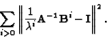
Each camera excluding the first, gives six constraints in eight unknowns, so three cameras are sufficient. In practice there are more than three cameras, and the non-linear least squares problem can be solved with Levenberg-Marquardt minimization algorithm [12]. As noticed in the case of Kruppa equations, a good initial guess for the unknowns ${\bf A}$ and ${\bf a}$ is needed in order for the algorithm to converge to the solution.

Given that from ${\bf H}^i_\infty$ the computation of ${\bf A}$ is straightforward, a guess for ${\bf a}$ (that determines ${\bf H}^i_\infty$) is sufficient. The cheirality constraints [14] are exploited by Hartley to estimate the infinity plane homography, thereby obtaining an approximate affine (or quasi-affine) reconstruction.

Pollefeys and Van Gool

In this approach [37], a projective reconstruction is first updated to affine reconstruction by the use of the modulus constraint [30,38]: since the left-hand part of (31) is conjugated to a (scaled) rotation matrix, all eigenvalues must have equal moduli. Note that this holds if and only if intrinsic parameters are constant. To make the constraint explicit we write the characteristic polynomial:

$$\det({\bf Q}^i + {\bf q}^i {\bf a}^\top- \lambda {\bf I}) = l_3 \lambda^3 + l_2 \lambda^2 + l_1 \lambda + l_0 .$$ (39)

The equality of the roots of the characteristic polynomial is not easy to impose, but a simple necessary condition holds:

 

l₃ l₁³ = l₂³ l₀ . (40)

This yields a fourth order polynomial equation in the unknown ${\bf a}$ for each camera except the first, so a finite number of solutions can be found for four cameras. Some solutions will be discarded using the modulus constraint, that is more stringent than (40).

As discussed previously, autocalibration is achievable with only three views. It is sufficient to note that, given three cameras, for every plane homography, the following holds [30]:

$${\bf H}^{1,3} = {\bf H}^{2,3} {\bf H}^{1,2} .$$ (41)

In particular it holds for the infinity plane homography, so

$${\bf H}_{\infty}^{i,j} = {\bf H}_{\infty}^j {{\bf H}_{\inft... ...}^j {\bf a}^\top) ({\bf Q}^i+ {\bf q}^i {\bf a}^\top) ^{-1} .$$ (42)

In this way we obtain a constraint on the plane at infinity for each pair of views. Let us write the characteristic polynomial:

 

$$\det(({\bf Q}^j+ {\bf q}^j {\bf a}^\top) ({\bf Q}^i+{\bf q}^i {\bf a}^\top) ^{-1} - \lambda {\bf I}) = 0 \iff$$ (43)

$$\det(({\bf Q}^j+ {\bf q}^j {\bf a}^\top) - \lambda ({\bf Q} ^i+{\bf q}^i {\bf a}^\top) ) =0$$ (44)

Writing the constraint (40) for the three views, a system of three polynomial of degree four in three unknowns is obtained. Here, like in the solution of Kruppa equations, homotopy continuation methods could be applied to compute all the 4³ = 64 solutions.

In practice more than three views are available, and we must solve a non-linear least-squares problem: Levenberg-Marquardt minimization is used by the author.

Heyden and Åström

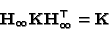
The method proposed by Heyden and Åström [20] is again based on (30), which can be rewritten as

$$\tilde{\bf P}^i_{\mathrm{proj}} \left [ \begin {array}{c} {\... ...\bf r}^\top\\ \end {array}\right] \simeq{\bf A} {\bf R}^i .$$ (45)

Since ${\bf R}^i {{\bf R}^i }^\top={\bf I}$ it follows that:

$$\tilde{\bf P}^i_{\mathrm{proj}} \left [ \begin {array}{c} {\... ...bf R}^i {{\bf R}^i }^\top{\bf A}^\top= {\bf A} {\bf A}^\top.$$ (46)

The constraints expressed by (46) are called the Kruppa constraints [20]. Note that (46) contains five equations, because the matrices of both members are symmetric, and the homogeneity reduces the number of equations with one. Hence, each camera matrix, apart from the first one, gives five equations in the eight unknowns $\alpha_u, \alpha_v, \gamma, u_0, v_0, r_1,r_2,r_3 .$A unique solution is obtained when three cameras are available. If the unknown scale factor is introduced explicitly, (46) rewrites:

$$0 = f_i({\bf A},{\bf r},\lambda_i) = \lambda_i^2 {\bf A} {\bf... ... \end {array}\right] \tilde{{\bf P}^i}^\top_{\mathrm{proj}} .$$ (47)

Therefore, 3 cameras yield 10 equations in 8 unknowns.

Triggs

Triggs [46] proposed a method based on the absolute quadric and, independently from Heyden and Åström, he derived an equation closely related to (46). The absolute quadric ${\pmb \Omega}$ consists of planes tangent to the absolute conic [6], and in a Euclidean frame, is represented by the matrix

$${\pmb \Omega}_\mathrm{euc} = \begin{bmatrix} {\bf I} & {\bf0}\\ {\bf0} &0 \end{bmatrix}.$$ (48)

If $\tilde{\bf T}$ is a projective transformation acting as in (25), then it can be verified [46] that it transforms ${\pmb \Omega}_\mathrm{euc}$ into ${\pmb \Omega} = \tilde{\bf T} {\pmb \Omega}_\mathrm{euc} \tilde{\bf T}^\top.$ Since the projection of the absolute quadric yields the dual image of the absolute conic [46], one obtain

$$\tilde{\bf P}^i_{\mathrm{proj}} {\pmb \Omega} \tilde{{\bf P}^i}^\top_{\mathrm{proj}} \simeq{\bf K}$$ (49)

from which, using (27), (46) follows immediately. Triggs, however, does not assume any particular form for $\tilde{\bf T}$, hence the unknown are ${\bf K}$ and ${\pmb \Omega}$. Note that both these matrix are symmetric and defined up to a scale factor.

Let ${\bf k}$ be the matrix composed by the the six elements of the lower triangle of ${\bf K}$, and ${\pmb \omega}$ be the matrix composed by the six elements of the lower triangle of $\tilde{\bf P}^i_{\mathrm{proj}} {\pmb \Omega} \tilde{{\bf P}^i}^\top_{\mathrm{proj}}$, then (49) is tantamount to saying that the two vectors are equal up to a scale, hence

$${\bf k} \wedge{\pmb \omega} = {\bf0}$$ (50)

in which the unknown scale factor is eliminated. For each camera this amounts to 15 bilinear equations in 9+5 unknowns, since both ${\bf k}$ and ${\pmb \omega}$ are defined up to a scale factor. Since only five of them are linearly independent, at least three images are required for a unique solution.

Triggs uses two methods for solving the non-linear least-squares problem: sequential quadratic programming [12] on $N \ge 3$ cameras, and a quasi-linear method with SVD factorization on $N \ge 4$ cameras. He recommend to use data standardization [15] and to enforce $\det({\pmb \Omega})=3$. The sought transformation $\tilde{\bf T}$ is computed by taking the eigen-decomposition of ${\pmb \Omega}$.

   
Bougnoux

This methods [4] is different from the previous ones, because it does not require constant intrinsic parameters and because it achieves only an approximate Euclidean reconstruction, without obtaining meaningful camera parameters as a by-product.

Let us write (25) in the following form:

$$\tilde{\bf P}^i_{\mathrm{eucl}} =\left[ \begin{array}{c\vert... ...ay}\right ]\simeq\tilde{\bf P}^i_{\mathrm{proj}}\tilde{\bf T}$$ (51)

where ${\bf q}_1^{i \top} ,{\bf q}_2^{i \top},{\bf q}_3^{i \top}$ are the rows of $\tilde{\bf P}^i_{\mathrm{eucl}} .$ The usual assumptions $\gamma = 0$ and $\alpha_u = \alpha_v$, are used to constraint the Euclidean camera matrices:

$$\gamma =0 \iff ( {\bf q}_1^i \wedge{\bf q}_3^i )^\top ({\bf q}_2^i \wedge{\bf q}_3^i ) =0$$ (52)

$$\alpha_u = \alpha_v \iff \vert\vert {\bf q}_1^i \wedge{\bf q}_3^i \vert\vert= \vert\vert {\bf q}_2^i \wedge{\bf q}_3^i \vert\vert.$$ (53)

Thus each camera, excluding the first, gives two constraints of degree four. Since we have six unknown, at least four cameras are required to compute $\tilde{\bf T}$. If the principal point (u₀, v₀) is forced to the image center, the unknowns reduce to four and only three cameras are needed.

The non-linear minimization required to solve the resulting system is rather unstable and must be started close to the solution: an estimate of the focal length and ${\bf r}$ is needed. Assuming known principal point, no skew, and unit aspect ratio, the focal length $\alpha_u$ can be computed from the Kruppa equations in closed form [4]. Then, given the intrinsic parameters ${\bf A}$, an estimate of ${\bf r}$ can be computed by solving a linear least-squares problem. From (46) the following is obtained:

$${\bf Q}^i {\bf A}{\bf A}^\top{\bf Q}^{i ^\top} + {\bf Q}^i {\... ... {\bf q}^i {\bf q}^{i ^\top} = \lambda^2 {\bf A} {\bf A}^\top.$$ (54)

Since $[{\bf A} {\bf A}^\top]_{3,3}={\bf K}_{3,3}=1,$ then $\lambda$ is fixed. After some algebraic manipulation [4], one ends up with four linear equations in ${\bf Ar}$. This method works also with varying intrinsic parameters, although, in practice, only the focal length is allowed to vary, since principal point is forced to the image center and no skew and unit aspect ratio are assumed. The estimation of the camera parameters is inaccurate, nevertheless Bougnoux proves that the reconstruction is correct up to an anisotropic homotethy, which he claims to be enough for the reconstructed model to be usable.

Discussion

Methods based on stratification have appeared only recently, and only preliminary and partial results are available. In many cases they show a graceful degradation as noise increases, but the issue of initialization is not always addressed. Hartley's algorithm leads to a minimization problem that requires a good initial guess; this is computed using a quite complicated method, involving the cheirality constraints. Pollefeys-VanGool's algorithm leads to an easier minimization, and this justify the claim that convergence toward a global minimum is relatively easily obtained. It is unclear, however, how the initial guess has to be chosen. The method proposed by Heyden and Åström  was evaluated only on one example, and was initialized close to the ground-truth. Experiments on synthetic data reported by Triggs, suggest that his non-linear algorithm is stable and requires only approximate initialization (the author reports that initial calibration may be wrong up to $50 \%$). Bougnoux's algorithm is quite different form the others, since its goal is not to obtain an accurate Euclidean reconstruction. Assessment of reconstruction quality is only visual.