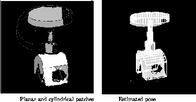
Figure 5: Estimating pose using Least Squares

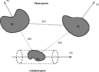
Figure 6: Geometric constraints on control points


[ Pose Estimation: Contents |
References ]


Figure 5, below, illustrates an example of 3D-3D pose estimation. The figure on the left shows depth data segmented into planar and cylindrical patches. The initial seed regions were found by curvature analysis and used as input to a robust (or a least squares) algorithm to find the best fitting surface to a set of data points defined by the curvature analysis. The control points used were the plane centres and the cylindrical axis centres (midway between the imaginary `caps' which fit on the ends of the cylindrical patch). The control vectors were the normals to the planes and the cylindrical axis vectors. Selection of which points to match was constrained by pairwise geometry, as illustrated in Figure 6. For example, the pair of vectors V1 and V2 and the separation of centres,d12 forms a rigid geometric quantity which is invariant to position in 3D space. If these vectors are measured, then they can index a pre-formed database which returns all pairs of planes of all models which have a similar configuration. By performing this for all scene entities, it is possible to obtain a prediction of which scene-model primitive correspondences occur most often. These should be should be used for pose prediction and verification.

Figure 5: Estimating pose using Least Squares

Figure 6: Geometric constraints on control points


[ Pose Estimation: Contents |
References ]