


Next: The Hough Transform
Up: Computer Vision IT412
Previous: Lecture 6
Subsections
It seems clear, both from biological and computational evidence, that
some form of data compression occurs at a very early stage in image
processing. Moreover, there is much physiological evidence suggesting
that one form of this compression involves finding edges and other
information-high features in images. Edges often occur at points where
there is a large variation in the luminance values in an image, and
consequently they often indicate the edges, or occluding boundaries,
of the objects in a scene. However, large luminance changes can also
correspond to surface markings on objects. Points of tangent
discontinuity in the luminance signal (rather than simple
discontinuity) can also signal an object boundary in the scene.
So the first problem encountered with modeling this biological process
is that of defining, precisely, what an edge might be. The
usual approach is to simply define edges as step discontinuities in
the image signal. The method of localising these discontinuities often then
becomes one of finding local maxima in the derivative of the signal,
or zero-crossings in the second derivative of the signal. This idea
was first suggested to the AI community, both biologically and
computationally, by Marr [5], and later developed by Marr and
Hildreth [6], Canny [1,2], and many others
[3,4].
In computer vision, edge detection is traditionally implemented by
convolving the signal with some form of linear filter, usually
a filter that approximates a first or second derivative operator.
An odd symmetric filter will approximate a first
derivative, and peaks in the convolution output will correspond to
edges (luminance discontinuities) in the image. An even symmetric
filter will approximate a second derivative operator. Zero-crossings
in the output of convolution with an even symmetric filter will
correspond to edges; maxima in the output of this operator will
correspond to tangent discontinuities, often referred to as
bars, or lines.
In this lecture we will begin by considering the classical
approaches to detecting edges in images: first derivative techniques,
second derivative techniques, and surface fitting. We will then
consider how features other than edges might be detected.
Most edge detection methods work on the assumption that an edge occurs
where there is a discontinuity in the intensity function or a very
steep intensity gradient in the image. Using this assumption, if we
take the derivative of the intensity values across the image and
find points where the derivative is a maximum, we will have marked
our edges.
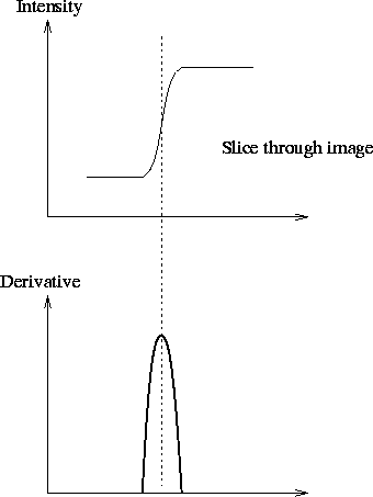
Figure 1:
An ideal step edge and its derivative profile.
 |
In a discrete image of pixels we can calculate the gradient by simply
taking the difference of grey values between adjacent pixels.
Figure 2:
An ideal step edge and its derivative profile.
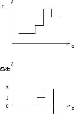 |
This is equivalent to convolving the image with the mask [-1,1].
Note that we have a problem in determining where we place the result of the
convolution. Ideally we would like to place it between the two
pixels. By using a mask that spans an odd number of pixels we end up
with a middle pixel to which we can assign the convolution result.
The gradient of the image function I is given by the
vector
![\begin{displaymath}
\nabla I = [\frac{\partial I}{\partial x}, \frac{\partial I}{\partial y}]. \end{displaymath}](img3.gif)
The magnitude of this gradient is given by
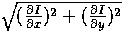 and its direction by
 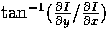 . Note, one can use any
pair of orthogonal directions to compute this gradient, although it is
common to use the x and y directions.
. Note, one can use any
pair of orthogonal directions to compute this gradient, although it is
common to use the x and y directions.
The simplest gradient operator is the Robert's Cross operator and
it uses the masks
![\begin{displaymath}
\begin{array}
{ccc}
\left[ \begin{array}
{cc}
0 & 1 \\ -1 ...
...n{array}
{cc}
1 & 0 \\ 0 & -1\end{array} \right]. \end{array}\end{displaymath}](img6.gif)
Thus the Robert's Cross operator uses the diagonal directions to calculate
the gradient vector.
A  approximation to
  is
given by the convolution mask
is
given by the convolution mask
This defines for
the Prewitt operator, and it detects vertical
edges.
The Sobel operator is a variation on this theme giving
more emphasis to the centre cell. The Sobel approximation to
is given by
Similar masks are constructed to approximate  ,thus detecting the horizontal component of any edges. Both the Prewitt and
Sobel edge detection algorithms convolve with masks to detect both the
horizontal and vertical edge components; the resulting outputs are simply
added to give a gradient map. The magnitude of the
gradient map is calculated and then input to a routine
that suppresses (to zero) all but the local maxima. This is known as
non-maxima suppression. The resulting map of local maxima is
thresholded (small local maxima will result from noise in the signal)
to produce the final edge map. It is the non-maxima suppression and
thresholding that introduce non-linearities into this edge detection
scheme. Moreover, the output of the thresholding stage is extremely sensitive
and there are no automatic procedures for satisfactorily determining thresholds
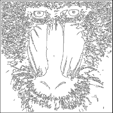
that work for all images. This is evident from the edge maps of
the mandrill image shown below.
,thus detecting the horizontal component of any edges. Both the Prewitt and
Sobel edge detection algorithms convolve with masks to detect both the
horizontal and vertical edge components; the resulting outputs are simply
added to give a gradient map. The magnitude of the
gradient map is calculated and then input to a routine
that suppresses (to zero) all but the local maxima. This is known as
non-maxima suppression. The resulting map of local maxima is
thresholded (small local maxima will result from noise in the signal)
to produce the final edge map. It is the non-maxima suppression and
thresholding that introduce non-linearities into this edge detection
scheme. Moreover, the output of the thresholding stage is extremely sensitive
and there are no automatic procedures for satisfactorily determining thresholds
that work for all images. This is evident from the edge maps of
the mandrill image shown below.
Figure 3:
The mandrill image.
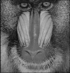 |
Figure 4:
The output of various edge detectors on the mandrill image.
Note that the use of default thresholds renders output that is
next to useless.
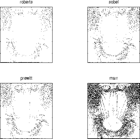 |
Figure 5:
The output of the Roberts and the Marr-Hildreth operators
on the scissors image. Note that edge contours are closed in the latter.
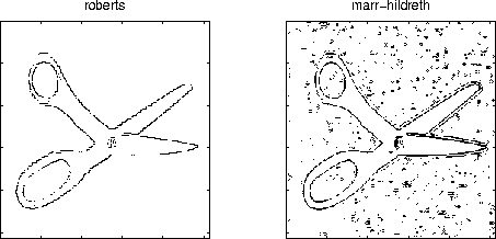 |
The main problem one has to deal with in differential edge detection
schemes is noise. The spikes in the derivative from the noise can mask
the real maxima that indicate edges. If we smooth the image then the
effects of noise can be reduced.
Figure 6:
A noisy step edge and its derivative (top); the smoothed signal
and its derivative (bottom).
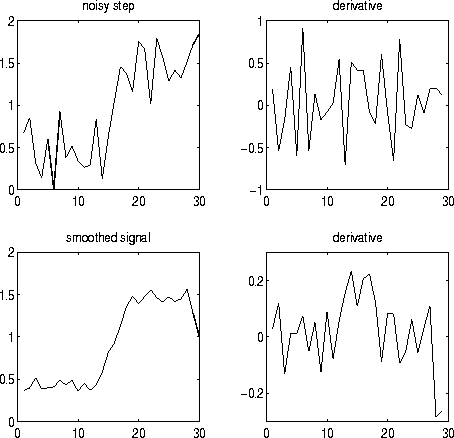 |
A procedure we could use is
- 1.
- Convolve the image with a Gaussian mask to smooth it, then
- 2.
- calculate derivatives of the smoothed image.
Both these operations are linear, and we can combine them in a different,
more computationally efficient way. If we calculate the derivative of
the Gaussian mask and convolve the image with this mask we compute the
derivative of the smoothed image in one hit. That is
where I is the image and G is the Gaussian mask.
A maximum of the first derivative will occur at a zero crossing of the
second derivative.
To get both horizontal and vertical edges we look at second derivatives
in both the x and y directions. This is the Laplacian of I
The Laplacian is linear and rotationally symmetric.
Thus, we search for the zero crossings of the image that
is first smoothed with a Gaussian
mask and then the second derivative is calculated; or
we can convolve the image with
the Laplacian of the Gaussian, also known as the LoG operator;
This defines the Marr-Hildreth operator.
Figure 7:
A Gaussian, its first and second derivatives, and the
DoG operator. Note that the 1st derivative is directionally
sensitive.
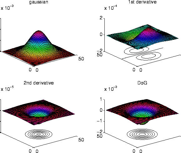 |
One can also get a shape similar to G'' by taking the difference of two
Gaussians having different standard deviations. A ratio of standard
deviations of 1:1.6 will give a close approximation to  .This is known as the DoG operator (Difference of Gaussians), or
the Mexican Hat Operator.
.This is known as the DoG operator (Difference of Gaussians), or
the Mexican Hat Operator.
The Marr-Hildreth operator became widely used for the following reasons:
- 1.
- Marr had considerable reputation.
- 2.
- Researchers found receptive fields in the eyes of animals (usually cats
and macaque monkeys) that behaved just like this operator.
- 3.
- The operator is symmetric. Edges are found in all orientations,
unlike the first derivative operators which are directional.
- 4.
- Zero crossings of the second derivative are simpler
to determine than are maxima in the first derivative; all that
needs to be done is to look for a sign change in the signal. Moreover,
the zero crossings of a signal always form closed contours.
This is nice if one is trying to separate out objects in the scene.
There are some problems, however.
- 1.
- Being a second derivative operator the influence of noise is
considerable.
- 2.
- Animals have lots of other types of receptive fields so this is not
the whole story.
- 3.
- Always generating closed contours is not realistic.
- 4.
- The Marr-Hildreth operator
will mark edges at some locations that are not edges.
The current standard edge detection scheme widely used around the
world is the Canny edge detector. This is the work John Canny
did for his Masters degree at MIT in 1983. He treated
edge detection as a signal processing problem and aimed
to design the `optimal' edge detector. He formally specified
an objective function to be optimised and used this to design the
operator.
The objective function was designed to achieve the following
optimisation constraints:
- 1.
- Maximize the signal to noise ratio to give good detection.
This favours the marking of true positives.
- 2.
- Achieve good localization to accurately mark edges.
- 3.
- Minimize the number of responses to a single edge. This favours the
identification of true negatives, that is, non-edges are not marked.
Note a difference-of-boxes operator will maximize the signal to noise ratio,
but will give several responses to a single edge.
After some complicated analysis Canny came up with a
function that was the sum of 4 exponential terms. However, this
function looked very much like a first derivative of a Gaussian! So
this is what ended up being used.
The overall edge detection procedure he developed was as follows:
- 1.
- We want to find the maxima of the partial derivative
of the image function I in the direction orthogonal to the edge
direction, and to smooth the signal along the edge direction.
Thus Canny's operator looks for the maxima of

where  However, many implementations of the Canny edge detector
actually approximate this process by first convolving the image with a Gaussian
to smooth the signal, and then looking for maxima in the first
partial derivatives of the resulting signal (using masks similar to
the Sobel masks).
Thus we can convolve the image with 4 masks, looking for horizontal, vertical
and diagonal edges. The direction producing the
largest result at each pixel point is marked. Record the convolution
result and the direction of the edge at each pixel.
However, many implementations of the Canny edge detector
actually approximate this process by first convolving the image with a Gaussian
to smooth the signal, and then looking for maxima in the first
partial derivatives of the resulting signal (using masks similar to
the Sobel masks).
Thus we can convolve the image with 4 masks, looking for horizontal, vertical
and diagonal edges. The direction producing the
largest result at each pixel point is marked. Record the convolution
result and the direction of the edge at each pixel.
- 2.
- Perform non-maximal suppression. Any gradient value that is not a
local peak is set to zero. The edge direction is used in this
process.
- 3.
- Find connected sets of edge points and form into lists.
- 4.
- Threshold these edges to eliminate `insignificant' edges. Canny
introduced the idea of thresholding hysteresis. This involves having
two different threshold values, usually the higher threshold being 3 times
the lower.
Any pixel in an edge list that has a gradient greater than the higher
threshold value are classed as a valid edge point. Any pixels
connected to these valid edge points that have a gradient
value above the lower threshold value are also classed as edge points.
That is, once you have started an edge you don't stop it until the gradient
on the edge has dropped considerably.
Figure 8:
The output of the Canny edge detector on the mandrill image.
Note that double edges are marked for line features.
 |
Gradient-based edge detection schemes suffer from a number of problems,
but they are still the most commonly used by the computer vision community.
Some of these problems include the following:
- 1.
- You have to choose threshold values and the width of your masks.
This problem is common to all gradient based methods. Note that if you
double the size of an image leaving its grey values unchanged all the
gradients will be halved. This complicates the setting of any
threshold. An additional problem is that the width of the mask (and
hence the degree of smoothing) affects the positions of zero crossings and
maximum intensity gradients in the image. The estimated position of
any edge should not be affected by the size of the convolution mask.
- 2.
- Corners are often missed because the 1D gradient at corners
is usually small.
This can cause considerable difficulties for line labeling schemes
because they rely on having corners and junctions being marked
properly.
- 3.
- First derivative operators will only find step-like features.
If you want to find lines you need a different operator. For example,
to find bar features you
could look for peaks (not zero crossings) from a second
derivative operator.
Canny did design an operator for finding lines.
Thus, differential edge detection schemes suffer both from false positives
and false negatives.
An alternative approach to edge detection is to develop an edge model
and then to compute its degree of match to the image data. In general,
though, surface fitting is computationally more expensive than
differential approaches to edge detection.
An edge is modeled by specifying its four degrees of freedom: its
position, its orientation, and the constant intensities on either side
of the step. We could simply match the data by seeking the least
squares error fit of the parametric model to the image window, but
such an approach is generally computationally very expensive.
Normally what is done is that both the image data and the model are
represented over small windows by their first 8 coefficients
in a particular two-dimensional orthonormal series expansion. In this
case the optimisation reduces to just one variable: the orientation
of the edge. An edge is declared present when the weighted least
squares error is smaller than some pre-set threshold.
Edge detector performance
A number of researchers have considered the problem of measuring
edge detector performance. In fact, it is difficult since we don't really
know what the underlying features are that we wish to detect. However, if we
assume that they are step edges corrupted by Gaussian noise, then some criteria
can be set for evaluating performance. Such criteria are usually the following:
- the probability of false edges;
- the probability of missing edges;
- the error in estimating the edge angle;
- the mean square distance of the edge estimate from the true edge; and
- the algorithm's tolerance to distorted edges and other features such
as corners and junctions.
The first two criteria relate to edge detection, the second two to edge
localisation, and the last to tolerance to departures from the
ideal edge model. Pratt [8] introduce$
function FM for measuring quantitatively the performance
of various edge detectors. His measure is
|
FM = |
1
| |
IA
å
i = 1
|
|
1
1 + di a2
|
, |
|
where IA, II, d, and a are respectively the detected edges,
the ideal edges, the distance between the actual and the ideal
edges, and a design constant used to penalise displaced edges.
Next: The Hough Transform
Up: Computer Vision IT412
Previous: Lecture 6
Robyn Owens
10/29/1997