Let us consider a signal f(t)=[1; 2; 3; 4; 4; 1; 1; 1; 2; 4; 5; 4; 3; 2; 1]. Let us consider an irregular sampling of this signal ![]() , where the missing samples have been replaced by zeroes. The associated certainty map will therefore be c(t)=[1; 0; 1; 1; 0; 1; 0; 1; 0; 1; 1; 0; 0;0;1], which indicates also the sampling grid. Let us consider the smoothing filter
, where the missing samples have been replaced by zeroes. The associated certainty map will therefore be c(t)=[1; 0; 1; 1; 0; 1; 0; 1; 0; 1; 1; 0; 0;0;1], which indicates also the sampling grid. Let us consider the smoothing filter ![]() .
.
In Figure 1 it is possible to see the approximation of the original signal f(t) (in blue) obtained by using the Normalized Convolution (in orange). The approximation of the signal obtained by Normalized Convolution is compared with the approximation which is possible to obtain from the same number of regularly spaced samples of the signal, using the inverse Discrete Fourier transform (IDFT) in order to obtain an approximation of the signal (in magenta). The reconstruction obtained with the normalized convolution is clearly superior.
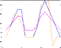
Figure 1: Reconstructed signal using the inverse Fourier Transform (IDFT) (in magenta) of the original signal (in blue) and the reconstruction of the signal obtained by Normalized Convolution (in orange).