The major drawback to threshold-based approaches is that they often lack the sensitivity and specificity needed for accurate classification. Sensitivity is defined as the true positive rate (TPR) for a function or a test that must detect the presence or absence of some intrinsic property (for example, tissue type) [74]. Hence, the purpose of the test is to determine, as accurately as possible, the presence or absence of this intrinsic property. Formally, the sensitivity of a binary test is defined as follows:
where True+ is defined as the number of samples that have the intrinsic property and were categorized by the test as positive, and Intrinsic+ is defined as the total number of elements that have the intrinsic property (regardless of the outcome of the test).
In the previous example, the simple threshold rule for classifying
bone will read the intensity values of each data element and
categorize it as true if the value is above the threshold ![]() and false if it is not above the threshold. Hence, this
test tries to determine an intrinsic property of an image pixel (i.e.,
bony = true or bony = false). In
Figure
and false if it is not above the threshold. Hence, this
test tries to determine an intrinsic property of an image pixel (i.e.,
bony = true or bony = false). In
Figure ![]() , the area under the Bone curve and to the
right of the Bone Threshold line is classified as T+
because this test will correctly categorize such elements as being
bone. The area under the Bone curve and to the left of the
Bone Threshold line is classified as F- because this test will
incorrectly classify such elements as not being bone. In this
example, the sensitivity is a measure of how well this test can
categorize as bone those tissues that are truly bone.
, the area under the Bone curve and to the
right of the Bone Threshold line is classified as T+
because this test will correctly categorize such elements as being
bone. The area under the Bone curve and to the left of the
Bone Threshold line is classified as F- because this test will
incorrectly classify such elements as not being bone. In this
example, the sensitivity is a measure of how well this test can
categorize as bone those tissues that are truly bone.
On the other hand, specificity is defined as the complement of the false positive rate (FPR):
where False- is defined as the total number of samples that do not have the intrinsic value but were categorized incorrectly as true, and Intrinsic- is defined as the total number of elements that do not have the intrinsic property [74].
In Figure ![]() , the area under the Muscle curve that
lies to the right of the Bone Threshold line is classified as
F+ because this test will incorrectly categorize such elements
as being bone. Conversely, the area under the Bone curve that lies to
the left of the Bone Threshold line is classified as
F- because this test will correctly categorize such elements as
not being bone. The specificity of this test is a measure of how well
this test will reject from the bone category those elements that truly
are not bone. Because their denominators are different, the
sensitivity and specificity measures are not complements of one
another. In fact, they measure two distinct aspects of any binary
test: the ability to correctly reject false properties and the ability
to correctly accept true properties.
, the area under the Muscle curve that
lies to the right of the Bone Threshold line is classified as
F+ because this test will incorrectly categorize such elements
as being bone. Conversely, the area under the Bone curve that lies to
the left of the Bone Threshold line is classified as
F- because this test will correctly categorize such elements as
not being bone. The specificity of this test is a measure of how well
this test will reject from the bone category those elements that truly
are not bone. Because their denominators are different, the
sensitivity and specificity measures are not complements of one
another. In fact, they measure two distinct aspects of any binary
test: the ability to correctly reject false properties and the ability
to correctly accept true properties.
It is important to realize that the definitions for sensitivity and specificity are valid for any test that performs binary categorization. No matter how sophisticated a test may be, it is still valid to ask what its sensitivity and specificity are.
As a rule, increasing the sensitivity of a binary test will reduce the
specificity of the test, and vice versa. For example, by increasing
the Bone Threshold in Figure ![]() , we can increase
the specificity of the test because there will be fewer false
positives. As a result, this will decrease the sensitivity because
there will be fewer true positives. By plotting specificity versus
sensitivity for a given test, we can construct what is known as a
Receiver Operator Characteristic (ROC) Curve [74]. The
ROC curve is a graphical representation of the trade-off between
specificity and sensitivity for a given test (see
Figure
, we can increase
the specificity of the test because there will be fewer false
positives. As a result, this will decrease the sensitivity because
there will be fewer true positives. By plotting specificity versus
sensitivity for a given test, we can construct what is known as a
Receiver Operator Characteristic (ROC) Curve [74]. The
ROC curve is a graphical representation of the trade-off between
specificity and sensitivity for a given test (see
Figure ![]() ). We can see by examining
Figure
). We can see by examining
Figure ![]() that increasing the sensitivity will cause the
specificity to decrease (more false positives).
that increasing the sensitivity will cause the
specificity to decrease (more false positives).

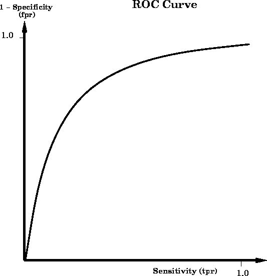
Figure: A Receiver Operator Characteristic (ROC) curve for the
simple bone classification test constructed by varying the bone
discriminating threshold. Points near the top right region of the
curve correspond to lower bone threshold values, whereas points
near the bottom left region of the curve correspond to higher bone
threshold values. Note that the vertical axis represents (1 -
Specificity), which is also known as the false positive rate
(fpr).
In addition to depicting the trade-off between specificity and
sensitivity for a given test, the ROC curve is also useful for
comparing the performance of different tests on the same
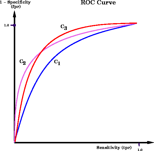
categorization tasks. For instance, suppose we had three tests (test
1, 2, and 3) that used three different techniques for categorizing
bone. By overlaying the ROC curves for each of the tests on the same
graph, we can visually determine which test performs better under
various conditions. For example, in Figure ![]() ,
the test depicted by curve
,
the test depicted by curve ![]() lies above and to the left of curve
lies above and to the left of curve
![]() . Hence, we conclude that test 3 is better than test 1 because
for any given value of sensitivity, test 3 has a lower false positive
rate (i.e., higher specificity). In practice, test 3 may be
undesirable for reasons other than its power of discrimination. For
example, test 1 may be a low-cost screening test for tuberculosis that
will be given to a large population, whereas test 3 may be a more
expensive chest X-ray exam. For a screening test, it is generally
better to trade specificity for increased sensitivity so that fewer
cases go undetected. The comparisons between test 1 and test 2 are
less clear. Although test 1 is better than test 2 for high values of
specificity, test 2 is better than test 1 for high values of
sensitivity. In the absence of any other considerations, test 2 would
be preferred in those situations where high sensitivity is preferred
(for example, screening tests), whereas test 1 would be preferred in
those situations where high specificity is preferred (for example, for
ruling out a diagnosis for a risky surgical procedure).
. Hence, we conclude that test 3 is better than test 1 because
for any given value of sensitivity, test 3 has a lower false positive
rate (i.e., higher specificity). In practice, test 3 may be
undesirable for reasons other than its power of discrimination. For
example, test 1 may be a low-cost screening test for tuberculosis that
will be given to a large population, whereas test 3 may be a more
expensive chest X-ray exam. For a screening test, it is generally
better to trade specificity for increased sensitivity so that fewer
cases go undetected. The comparisons between test 1 and test 2 are
less clear. Although test 1 is better than test 2 for high values of
specificity, test 2 is better than test 1 for high values of
sensitivity. In the absence of any other considerations, test 2 would
be preferred in those situations where high sensitivity is preferred
(for example, screening tests), whereas test 1 would be preferred in
those situations where high specificity is preferred (for example, for
ruling out a diagnosis for a risky surgical procedure).

Figure: A family of ROC curves for a hypothetical set of
classifiers. Test 1 (represented by ![]() ) is a better classifier
than tests 2 and 3 because for all values of sensitivity, test 1
has a lower false positive rate. Test 2 is better than test 3
only at high values of sensitivity.
) is a better classifier
than tests 2 and 3 because for all values of sensitivity, test 1
has a lower false positive rate. Test 2 is better than test 3
only at high values of sensitivity.