Orthogonal Complex Zernike Moments

Complex Zernike moments [5] are constructed using a set of complex polynomials which form a complete orthogonal basis set defined on the unit disc $x^{2} + y^{2} \leq 1$. They are expressed as:

$$A_{mn} = \frac{m+1}{\pi} \int \int_{x^{2} + y^{2} \leq ~1} f(x,y)[V_{mn}(x,y)]^{*} ~dx~dy$$ (1)

where $m = 0,1,2...\infty$, $f(x,y)$ is the function being described, $*$ denotes the complex conjugate and $n$ is an integer, subject to the conditions:

$$m- \mid n \mid ~=~even~~,~~\mid n \mid~\leq~m$$ (2)

The Zernike polynomials [2] $V_{mn}(x,y)$, expressed in polar coordinates are:

$$V_{mn}(r,\theta)~=~R_{mn}(r)\exp(jn\theta)$$ (3)

where $(r,\theta)$ are defined over the unit disc and $R_{mn}(r)$ is the orthogonal radial polynomial, defined as:

$$R_{mn}(r) = \sum_{s=0}^{\frac{m-\mid~n~\mid}{2}}(-1)^{s}~~F(m,n,s,r)$$ (4)

where:

$$F(m,n,s,r) = \frac{(m-s)!}{s!(\frac{m+\mid~n~\mid}{2}~-s)!~(\frac{m-\mid~n~\mid}{2}~-s)! }~r^{m-2s}$$ (5)

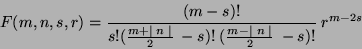
The first six orthogonal radial polynomials are:

$$R_{00}(r) = 1~~ ~~R_{11}(r) = r$$ (6)

$$R_{20}(r) = 2r^{2} - 1~~ ~~ R_{22}(r) = r^{2}$$

$$R_{31}(r) = 3r^{3} - 2r~~ ~~R_{33}(r) = r^{3}$$

Figure 1 shows eight such radial responses, where it can been seen that the polynomials become more grouped, as they approach the edge of the unit disc.

Figure 1: Eight orthogonal radial polynomial plots.

So for a discrete image, if $P(x,y)$ is the current pixel then Equation 1 becomes :

$$A_{mn} = \frac{m+1}{\pi} \sum_{x} \sum_{y} P(x,y)[V_{mn}(x,y)]^{*} ~~~~~\mbox{where $x^{2} + y^{2} \leq ~1$}$$ (7)

To calculate the Zernike moments of an image $f(x,y)$, the image (or region of interest) is first mapped to the unit disc using polar coordinates, where the centre of the image is the origin of the unit disc. Those pixels falling outside the unit disc are not used in the calculation. The coordinates are then described by $r$ which is the length of the vector from the origin to the coordinate point and $\theta$ which is the angle from the $x$ axis to the vector $r$, by convention measured from the positive $x$ axis in a counter clockwise direction. The mapping from Cartesian to polar coordinates is:

$$x = r~\cos\theta~~~~~~~~y = r~\sin\theta$$ (8)

where

$$r = \sqrt{x^2 + y^2} ~~~~~~~~ \theta = \tan^{-1}\left(\frac{y}{x}\right)$$ (9)

However, $\tan^{-1}A$ in practice is often defined over the interval $- \frac{\pi}{2} \leq \theta \leq \frac{\pi}{2}$, so care must be taken as to which quadrant the Cartesian coordinates appear in. Translation and scale invariance can be achieved by normalising the image using the Cartesian moments prior to calculation of the Zernike moments [1]. Translation invariance is achieved by moving the origin to the centre of the image by using the centralised moments, causing $m_{01}=m_{10}=0$. Following this, scale invariance is produced by altering each object so that its area (or pixel count for a binary image) is $m_{00}=\beta$, where $\beta$ is a predetermined value. Both invariance properties can be achieved using :

$$g(x,y) = f \left( \frac{x}{a} + \overline{x},\frac{y}{a} + \... ...y} \right) ~~~~~\mbox{where $a = \sqrt{\frac{\beta}{m_{00}}}$}$$ (10)

and $g(x,y)$ is the new translated and scaled function. The error involved in the discrete implementation can be reduced by interpolation. If the coordinate calculated by Equation 10 does not coincide with an actual grid location, the pixel value associated with it is interpolated from the four surrounding pixels. As a result of the normalisation, the Zernike moments $\mid A_{00} \mid$ and $\mid A_{11} \mid$ are set to known values. $\mid A_{11} \mid$ is set to zero, due to the translation of the shape to the centre of the coordinate system. This however will be affected by a discrete implementation where the error will decrease as the image size increases. $\mid A_{00} \mid$ is dependent on $m_{00}$, and thus on $\beta$:

$$\mid A_{00} \mid ~= \frac{\beta}{\pi}$$ (11)

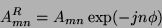
Further, the absolute value of a Zernike moment is rotation invariant as reflected in the mapping of the image to the unit disc. The rotation of the shape around the unit disc is expressed as a phase change, if $\phi$ is the angle of rotation, $A_{mn}^R$ is the Zernike moment of the rotated image and $A_{mn}$ is the Zernike moment of the original image then:

$$A_{mn}^R = A_{mn}\exp(-jn\phi)$$ (12)