Zernike Velocity Moments

The new Zernike velocity moments [3] are expressed as:

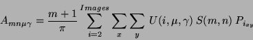$$A_{mn\mu\gamma} = \frac{m+1}{\pi} \sum^{Images}_{i=2} \sum_{... ...)~S(m,n)~P_{i_{xy}} %%~~~~~~~~~~\mbox{$x^{2} + y^{2} \leq ~1$}$$ (19)

They are bounded by $x^{2} + y^{2} \leq 1$, while the shape's structure contributes through the orthogonal polynomials:

$$S(m,n)~=~[V_{mn}(r,\theta)]^{*}$$ (20)

Velocity is introduced as before (Equation 15), while normalisation is produced by:

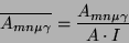$$\overline{A_{mn\mu\gamma}} = \frac{A_{mn\mu\gamma}}{A\cdot I}$$ (21)

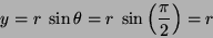
The coordinate values for $U(i,\mu,\gamma)$ are calculated using the Cartesian moments and then translated to polar coordinates. If we consider first the $x$ direction case only, from Equation 8 the angle $\theta$ for a difference in $x$ position is either $0$ or $\pi$ radians. The value used is dependent on the direction of movement. If the movement is in the positive $x$ direction (or left to right) then:

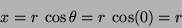$$x = r~\cos\theta = r~\cos(0) = r$$ (22)

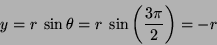
where $r$ is the length of the vector from the previous COM (Centre of Mass - as defined by the first order Cartesian moment) to the current COM, ie the velocity in pixels/image. Alternatively, if the movement is in the negative $x$ direction (or right to left) then:

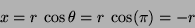$$x = r~\cos\theta = r~\cos(\pi) = -r$$ (23)

The mapping to polar coordinates results in a sign change which could be used to detect the direction of motion. Similarly for the $y$ direction velocity, the values of $\theta$ are either $\frac{\pi}{2}$ or $\frac{3\pi}{2}$ radians, and using Equation 8 produces:

$$y = r~\sin\theta = r~\sin\left(\frac{\pi}{2}\right) = r$$ (24)

and

$$y = r~\sin\theta = r~\sin\left(\frac{3\pi}{2}\right) = -r$$ (25)