


Next: Bibliography
Up: CVonline_ANOVA
Previous: CVonline_ANOVA
One way ANOVA - Analysis of variance
Analysis of variance (ANalysis Of VAriance) is a general method for studying sampled-data relationships [1,2].
The method enables the difference between two or more sample means to be analysed, achieved by subdividing the total sum of squares.
One way ANOVA is the simplest case. The purpose is to test for significant differences between class means, and this is done by analysing the variances. Incidentally, if we are only comparing two different means then the method is the same as the  for independent samples. The basis of ANOVA is the partitioning of sums of squares into between-class (
 ) and within-class (
 ). It enables all classes to be compared with each other simultaneously rather than individually; it assumes that the samples are normally distributed.
The one way analysis is calculated in three steps, first the sum of squares for all samples, then the within class and between class cases. For each stage the degrees of freedom
). It enables all classes to be compared with each other simultaneously rather than individually; it assumes that the samples are normally distributed.
The one way analysis is calculated in three steps, first the sum of squares for all samples, then the within class and between class cases. For each stage the degrees of freedom  are also determined, where is the number of independent `pieces of information' that go into the estimate of a parameter. These calculations are used via the Fisher statistic to analyse the null hypothesis. The null hypothesis states that there are no differences between means of different classes, suggesting that the variance of the within-class samples should be identical to that of the between-class samples (resulting in no between-class discrimination capability). It must however be noted that small sample sets will produce random fluctuations due to the assumption of a normal distribution.
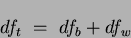
If
are also determined, where is the number of independent `pieces of information' that go into the estimate of a parameter. These calculations are used via the Fisher statistic to analyse the null hypothesis. The null hypothesis states that there are no differences between means of different classes, suggesting that the variance of the within-class samples should be identical to that of the between-class samples (resulting in no between-class discrimination capability). It must however be noted that small sample sets will produce random fluctuations due to the assumption of a normal distribution.
If  is the sample for the
  class and
  data point then
the total sum of squares is defined as:
data point then
the total sum of squares is defined as:
 |
(1) |
with degrees of freedom:
 |
(2) |
where  is the number of data points (assuming equal numbers of data points in each class) and
  is the number of classes and
  is the grand mean:
 |
(3) |
The second stage determines the sum of squares for the within class case, defined as:
 |
(4) |
where  is the class mean determined by:
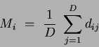 |
(5) |
and the within class is:
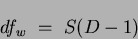 |
(6) |
The sum of squares for the between class case is:
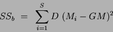 |
(7) |
with the corresponding of:
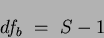 |
(8) |
Defining the total degrees of freedom  and the total sum of squares
  as:
as:
 |
(9) |
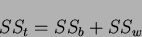 |
(10) |
Finally if  is the mean square deviations (or variances) for the between class case, and
  is the reciprocal for the within class case then:
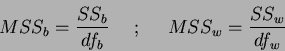 |
(11) |
It is now possible to evaluate the null hypothesis using the Fisher or  Fisher statistic statistic, defined as:
 |
(12) |
If  then it is likely that differences between class means exist. These results are then tested for statistical significance or
  -value, where the -value is the probability that
a variate would assume a value greater than or equal to the value observed strictly by chance.
If the -value is small (eg.
-value, where the -value is the probability that
a variate would assume a value greater than or equal to the value observed strictly by chance.
If the -value is small (eg.  or
or  ) then this implies that the means differ by more than would be expected by chance alone. By setting a limit on the -value, (i.e.
  ) a critical value can be determined. The critical value
  is determined (via standard lookup tables) through the between-class (
 ) and within-class (
 ) values. Values of greater than the critical value denote the rejection of the null hypothesis, which prompts further investigation into the nature of the differences of the class means. In this way ANOVA can be used to prune a list of features.
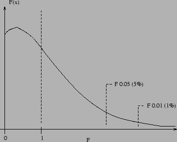
Figure 0.1 shows example Fisher statistic critical value values for a low distribution (i.e. a small dataset). As increases (i.e. the dataset size increases) the distribution will become `tighter' and more peaked in appearance, while the peak will shift away from the
) values. Values of greater than the critical value denote the rejection of the null hypothesis, which prompts further investigation into the nature of the differences of the class means. In this way ANOVA can be used to prune a list of features.
Figure 0.1 shows example Fisher statistic critical value values for a low distribution (i.e. a small dataset). As increases (i.e. the dataset size increases) the distribution will become `tighter' and more peaked in appearance, while the peak will shift away from the  axis towards
  .
.
Figure 0.1:
Example F distribution (for low ) showing possible  and intervals.
 |
The value gives a reliable test for the null hypothesis, but it cannot indicate which of the means is responsible for a significantly low probability. To investigate the cause of rejection of the null hypothesis post-hoc or multiple comparison tests can be used. These examine or compare more than one pair of means simultaneously.
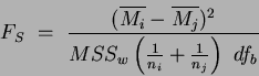
Here we use the Scheffe post-hoc test. This tests all pairs for differences between means and all possible combinations of means. The test statistic 
 Scheffe post-hoc test value is:
 |
(13) |
where  and
and  are the classes being compared and
  and are the number of samples and mean of class , respectively. If the number of samples (data points) is the same for all classes then
 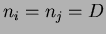 . The test statistic is calculated for each pair of means and the null hypothesis is again rejected if is greater than the critical value , as previously defined for the original ANOVA analysis.
This Scheffe post hoc test is known to be conservative which helps to compensate for spurious significant results that occur with multiple comparisons [2]. The test gives a measure of the difference between all means for all combinations of means.
. The test statistic is calculated for each pair of means and the null hypothesis is again rejected if is greater than the critical value , as previously defined for the original ANOVA analysis.
This Scheffe post hoc test is known to be conservative which helps to compensate for spurious significant results that occur with multiple comparisons [2]. The test gives a measure of the difference between all means for all combinations of means.
In terms of classification, large statistic values do not necessarily indicate useful features. They only indicate a well spread feature space, which for a large dataset is a positive attribute. It suggests that the feature has scope or `room' for more classes to be added to the dataset. Equally, features with smaller values (but greater than the critical values ) may separate a portion of the dataset, which was previously `confused' with another portion. Adding this new feature, increasing the feature space dimensions, may prove beneficial. In this manner, features which appear `less good' (i.e. lower statistic values than alternative features) may, in fact, prove useful in terms of classification.
Next: Bibliography
Up: CVonline_ANOVA
Previous: CVonline_ANOVA
Jamie Shutler
2002-08-15