 For this description, only noise processes with zero mean will be
considered (this is without loss of generality).
The Wiener filter is the MSE-optimal stationary linear filter for images
degraded by additive noise and blurring. Calculation of the Wiener
filter requires the assumption that the signal and noise processes
are second-order stationary (in the random process sense). For this description, only noise processes with zero mean will be
considered (this is without loss of generality).
Wiener filters are usually applied in the frequency domain. Given a degraded image x(n,m), one takes the Discrete Fourier Transform (DFT) to obtain X(u,v). The original image spectrum is estimated by taking the product of X(u,v) with the Wiener filter G(u,v):
![]()
The inverse DFT is then used to obtain the image estimate from its spectrum. The Wiener filter is defined in terms of these spectra:

The Wiener filter is:
![]()
Dividing through by ![]() makes its behaviour easier to explain:
makes its behaviour easier to explain:

The term ![]() can be interpreted as the reciprocal of the
signal-to-noise ratio. Where the signal is very strong relative
to the noise,
can be interpreted as the reciprocal of the
signal-to-noise ratio. Where the signal is very strong relative
to the noise, ![]() and the Wiener filter becomes
and the Wiener filter becomes
![]() - the inverse filter for the PSF. Where the signal
is very weak,
- the inverse filter for the PSF. Where the signal
is very weak, ![]() and
and ![]() .
.
For the case of additive white noise and no blurring, the Wiener filter simplifies to:
![]()
where ![]() is the noise variance.
is the noise variance.
Wiener filters are unable to reconstruct frequency components which have been degraded by noise. They can only suppress them. Also, Wiener filters are unable to restore components for which H(u,v)=0. This means they are unable to undo blurring caused by bandlimiting of H(u,v). Such bandlimiting occurs in any real-world imaging system.
Obtaining ![]() can be problematic. One can assume that
can be problematic. One can assume that ![]() has
a parametric shape, for example exponential or Gaussian. Alternately,
has
a parametric shape, for example exponential or Gaussian. Alternately,
![]() can be estimated using images representative of the class of
images being filtered. For Wiener results presented in this thesis,
can be estimated using images representative of the class of
images being filtered. For Wiener results presented in this thesis,
![]() was calculated from image to be filtered:
was calculated from image to be filtered: ![]() was assumed to
be radially symmetric,
i.e.
was assumed to
be radially symmetric,
i.e. ![]() and was estimated by averaging over
30 radial frequency bands. Linear interpolation was used to give
and was estimated by averaging over
30 radial frequency bands. Linear interpolation was used to give ![]() a smooth shape.
a smooth shape.

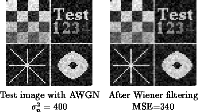
Figure 1.5: Example of Wiener filtering
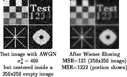
Figure 1.5 shows a Wiener filter result. The small test image has very strong high-frequency components, so the Wiener filter leaves lots of residual noise. If the test image, which is 64x64, is centered in a 256x256 empty image, the relative power of those high-frequency components is diminished by the large amounts of empty space. The Wiener filter then elects to attenuate high-frequency components to reduce noise in the empty regions. This results in blurring over the small 64x64 subimage (Figure 1.6). Although the MSE over the 256x256 image is quite small, the MSE over the 64x64 test region increases from 400 to 1232. This illustrates an important point about using MSE as a criteria for global filtering: regions are given priority for restoration according to how large they are, rather than their visual importance.

Figure 1.6: Another example of Wiener filtering
Wiener filters are comparatively slow to apply, since they require working in the frequency domain. To speed up filtering, one can take the inverse FFT of the Wiener filter G(u,v) to obtain an impulse response g(n,m). This impulse response can be truncated spatially to produce a convolution mask. The spatially truncated Wiener filter is inferior to the frequency domain version, but may be much faster.