This teach file deals with one method of finding specified shapes in images: the Hough transform.
Please read the introduction giving general information about the nature of this document.
You should have read the 3 previous teach files, VISION1, VISION2, VISION3. As usual, it will be helpful to get the necessary libraries loaded now, and to load a test image. It is particularly important, when working through this teach file, to run the examples in order, as they are more interdependent than usual.
    uses popvision          ;;; search vision libraries
    uses rci_show           ;;; image display
    uses rc_context         ;;; allows multiple windows for graphics
    uses rc_graphplot       ;;; graph drawing
    uses arrayfile          ;;; array storage
    uses float_byte         ;;; type conversion
    uses float_arrayprocs   ;;; array arithmetic
    uses canny              ;;; Canny edge detection
    uses straight_hough     ;;; Hough transform

    vars image;
    arrayfile(popvision_data dir_>< 'stereo1.pic') -> image;
    float_byte(image, false, false, 0, 255) -> image;
    false -> popradians;        ;;; this teach file uses°
It is useful to be able to find simple shapes - straight lines, circles, ellipses and the like - in images. Man-made objects, for instance, frequently have shapes with straight and circular edges, which project to straight and elliptical boundaries in an image. One kind of algorithm for identifying these extended image features involves following edges, and linking together edgelets which seem to lie on straight lines or smooth curves. An alternative approach, which is the subject of this teach file, involves accumulating the evidence provided by each edge element for the shape being sought. Since, usually, the shape can be at any position in the image, and often at any orientation and of any size as well, the whole set of different possibilities has to be taken into account.
The Hough transform is used in a variety of related methods for shape detection. These methods are fairly important in applied computer vision; in fact, Hough published his transform in a patent application, and various later patents are also associated with the technique.
To see how the methods work, we will take one of the simplest possible shapes as an example: the straight line. This is often a building block for higher-level descriptions of image structure, and a basis for matching in model-based vision.
A straight line in an image has two ends, but the Hough transform illustrated here does not find end-points. Rather it finds the infinite straight lines on which the image edges lie. A part of a line lying between two end-points is called a line segment, whilst in this file the term line will mean an infinite straight line. These infinite lines are worth extracting, since once found they can be followed through the image and end-points located.
Positions in images have been represented so far by coordinates corresponding to the column and row indices of array elements. Now it will be helpful to use a different coordinate system, with its origin in the centre of the image. We will call this the (x, y) coordinate system, and it will have y running up the screen and x running from left to right in the conventional way. The following code will illustrate these coordinates for you, with x and y each running from -100 to +100 pixels from the origin.
rc_new_window(300, 300, 550, 50, true); ;;; get a window
(If the size or position of the window is inconvenient, adjust it with the mouse now.)
    [-100 100 -100 100] -> rcg_usr_reg;     ;;; set image size
    rc_graphplot([], 'x', [], 'y') -> ;     ;;; draw axes
(In this file the *RC_GRAPHPLOT package is used to draw the axes and set the scales and origins of coordinate systems for the illustrations. This gives an easy way of making the axes correspond to the coordinate system for *RC_GRAPHIC commands. You do not need to bother with these details of the examples, unless you want to experiment further with these facilities - you should be able to see what is going on by looking at the graphics in the display windows.)
It is easy to translate between the (x, y) coordinates and array (column, row) coordinates.
There are various ways to specify a line. One method, particularly suited to the Hough transform, is as follows. Imagine yourself standing on the image plane at the origin of the coordinates, facing the positive x direction (to the right on the screen). Turn a specified angle to your left, and then walk a specified number of pixels forward. Turn through 90° and go forward; you are now walking along the required line in the image.
The following code illustrates this on the screen. Suppose you turn through 60° and walk 50 pixels forward. Then your path can be drawn with:
    XpwSetColor(rc_window, 'blue') -> ;     ;;; draw in blue
    rc_jumpto(0, 0);            ;;; start at the origin
    60 -> rc_heading;           ;;; face 60° left of x-axis
    rc_draw(50);                ;;; go 50 pixels
and then the line we are interested in with:
    XpwSetColor(rc_window, 'red') -> ;      ;;; draw in red
    rc_turn(90);                ;;; turn 90° left
    rc_draw(150);               ;;; draw some of the line
    rc_turn(180);               ;;; turn right round
    rc_draw(300);               ;;; draw the other way
    XpwSetColor(rc_window, 'black') -> ;      ;;; go back to black
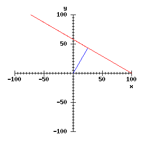
It should be clear that any line can be drawn by setting two quantities in this algorithm: the angle intially turned through, called theta, and the distance moved from the origin, called r. The red line is therefore the line with parameters r = 50 pixels, theta = 60°. It will be useful to incorporate the moves above into a procedure for drawing lines specified this way:
    define draw_rt_line(r, theta);
        ;;; Draw a line specified by r, theta
        lvars r, theta;
        lconstant lngth  = 300;           ;;; assume 300 long enough
        rc_jumpto(0, 0);            ;;; start at the origin
        theta -> rc_heading;        ;;; turn by theta
        rc_jump(r);                 ;;; move, do not draw
        rc_turn(90);                ;;; turn through 90
        rc_jump(lngth/2);           ;;; move along the line
        rc_turn(180);               ;;; face back along it
        rc_draw(lngth);             ;;; draw the line
    enddefine;
So the red line could be drawn with draw_rt_line(50, 60). If you are still unclear about the (r, theta) parameterisation of the line, use draw_rt_line to draw some more lines on the window.
You may have met other ways of describing lines, e.g. the (m, c) parameterisation, where m is the slope and c is the y-axis intercept, and the line has the equation y = mx + c. This is not so useful for our purposes, because for lines nearly parallel to the y-axis, m gets extremely large.
Suppose we have detected an image feature at particular (x, y) coordinates, perhaps using an edge detector. We will assume that we know the position of the feature, but that any orientation associated with it (e.g. the direction of the grey-level gradient) is not accurate enough to be useful. If we are looking for lines in the image, then a feature at a particular point is evidence that there might be a line passing through that point. Many different lines pass through a given point, and the feature is evidence for any or all of them, so we need a way of finding the set of lines through a point.
If we have a feature at (x, y), and we know the theta parameter of a line through the feature, then we can calculate the line's r parameter with this equation:
r = x cos(theta) + y sin(theta)
You might be able to check this statement with a little geometry and algebra, but it is not necessary to do so here; we can verify experimentally that it seems to hold. Suppose there is a feature at x = 30, y = 70. Clear the window and mark the feature with:
    rc_graphplot([], 'x', [], 'y') -> ;     ;;; just draw axes
    rc_jumpto(30, 70);                      ;;; go to x=30, y=70
    rc_point_here();                        ;;; draw a dot
The dot is probably almost invisible, so let's put a circle round it:
    0 -> rc_heading;                        ;;; face right
    rc_jump(5);                             ;;; move 5 pixels
    90 -> rc_heading;                       ;;; face top
    rc_arc_around(5, 360);                  ;;; draw circle
Now, arbitrarily choosing theta = 70°, we can draw a line through the feature by calculating r using the equation above, and then calling draw_rt_line. Thus:
    vars r, theta;
    70 -> theta;
    30 * cos(theta) + 70 * sin(theta) -> r; ;;; x=30, y=70
    XpwSetColor(rc_window, 'red') -> ;
    draw_rt_line(r, theta);
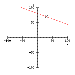
And it is easy enough now to draw as many lines as we like through the feature, particularly if the formula above is made into a procedure:
    define line_r(x, y, theta) -> r;
        lvars x, y, theta, r;
        x * cos(theta) + y * sin(theta) -> r
    enddefine;
    for theta from 0 by 10 to 350 do    ;;; lines at 10° intervals
        line_r(30, 70, theta) -> r;
        draw_rt_line(r, theta);
    endfor;
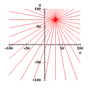
Clearly, we do not normally want to draw a lot of lines. What we do want to do is to record the set of lines in a data structure. To this end, it is useful to introduce a parameter space for lines. (This is sometimes called a Hough space.) A two-dimensional parameter space is just a plane for which the coordinates are the parameters. We can visualise the parameter space for r and theta in another window, set up like this:
    vars xy_context;                    ;;; save the present window
    rc_context(false) -> xy_context;    ;;; and its coord system
    false -> rc_window;
    rc_new_window(300, 300, 550, 400, true);
    [0 100 0 360] -> rcg_usr_reg;        ;;; bounds of parameter space
    rc_graphplot([], 'r', [], 'theta') -> ; ;;; draw axes
A point in this window is to correspond to a line in the x-y window we have used so far. Let us plot the points in parameter space that correspond to the lines we have drawn. This involves using almost the same code we had above. Instead of calling draw_rt_line, we just need to mark a point in parameter space - a simple procedure to draw a cross (from LIB *RCG_UTILS) is used to mark the points in the new window.
    XpwSetColor(rc_window, 'red') -> ;  ;;; draw in red
    for theta from 0 by 10 to 350 do    ;;; lines at 10° intervals
        line_r(30, 70, theta) -> r;
        rcg_plt_plus(r, theta);         ;;; draw a cross
    endfor;
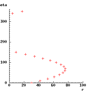
There appears to be one problem - some of the values of r were negative, so have vanished off the left of the graph. In fact, it is safe to ignore the negative values - an explanation of this follows later.
Suppose there is a second feature in the image, at, say, x = -50, y = 20. We can mark the parameters for the lines that pass through it as well, with:
    for theta from 0 by 10 to 350 do    ;;; lines at 10° intervals
        line_r(-50, 20, theta) -> r;
        rcg_plt_plus(r, theta);
    endfor;
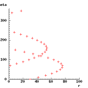
As you can see from the display, the two lines of crosses intersect at about r = 45, theta = 120°. These, then, must be the parameter values for a line that passes through both the two features. To check, the next piece of code switches back to the x-y window, marks the new feature, and then draws the line with the parameters r = 45, theta = 120°.
    vars rt_context;                ;;; to hold the r-theta window
    rc_context(false) -> rt_context; ;;; and save it
    xy_context -> rc_context();     ;;; go back to x-y window

    ;;; Mark the point at x=-50, y=20 with a circle - see above
    XpwSetColor(rc_window, 'black') -> ;
    rc_jumpto(-50, 20);
    rc_point_here();
    0 -> rc_heading;
    rc_jump(5);
    90 -> rc_heading;
    rc_arc_around(5, 360);

    XpwSetColor(rc_window, 'blue') -> ;     ;;; draw in blue
    draw_rt_line(45, 120);
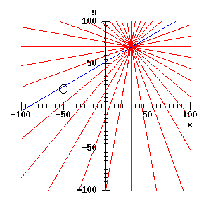
So we have found (approximately) the parameters of the line through the two features, via the parameter space representation. This is a most cumbersome way to find a line through two points, but it comes into its own if we have a large number of points to deal with - as with a processed image.
Suppose that we have a third feature, on almost the same line as the other two - say at x = 0, y = 50. Then its Hough space representation will intersect at the same point as the previous two:
    rt_context -> rc_context();
    for theta from 0 by 10 to 350 do
        line_r(0, 50, theta) -> r;
        rcg_plt_plus(r, theta);
    endfor;
whereas a point somewhere off the line (e.g. at x = 50, y = -50) will not contribute to the cluster near r = 45, theta = 120:
    XpwSetColor(rc_window, 'blue') -> ;
    for theta from 0 by 10 to 350 do
        line_r(50, -50, theta) -> r;
        rcg_plt_plus(r, theta);
    endfor;
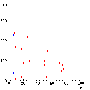
If more and more points that are on our line are detected, then more and more evidence will accumulate in the r = 45, theta = 120 region of the parameter space. Points that are not on the line will contribute to other parts of the space, but will not form a definite cluster unless they happen to lie on another straight line. If several straight lines are present, then several clusters will form in parameter space.
To detect lines in practice, we need to record where the points fall in parameter space. To do this, we use an array, called an accumulator array, such that elements of the array correspond to small regions of parameter space. To start with, every element of the accumulator array will be set to zero. For each point in parameter space to be recorded, the appropriate element of the array is incremented. An element of the accumulator array is sometimes called a bin.
Dividing parameter space up into regions for this purpose is known as quantisation. How many rows and columns to use in the accumulator array, that is, how to quantise parameter space, is an important issue - it is beyond this teach file, though it is fair to say that trial and error often play a large part.
We will use an accumulator array with column number corresponding to r and row number corresponding to theta. Suppose (somewhat arbitrarily) we use 100 bins along r and 100 along theta, numbering them from 0 to 99, giving 10,000 bins altogether. To get from r and theta to column and row in the accumulator array, we can use
    round(r) -> accumulator_column;
    round(theta/3.6) -> accumulator_row;
The round procedure returns the nearest integer to its argument. We can see that the quantisation interval is 1 pixel in r, and 3.6° in theta. You can imagine drawing a grid with lines separated by 3.6 units vertically and 1 unit horizontally on the parameter space window. All the crosses that fall into one cell of the grid will contribute to one element of the accumulator array.
The increments to a bin of the accumulator array are sometimes referred to as votes. Each edge element in the image votes for those bins in parameter space which represent lines that pass close to that element. It follows that the bins which get the most votes correspond to lines which have many edge elements lying close to them.
To see if this works, we will use data from a real image.
We will use edge data from the example at the end of TEACH *VISION3. Here is the code to get the edge map, and to display it:
    vars bin_edges;
    vars sigma = 1;         ;;; smoothing
    vars t1 = 5, t2 = 10;   ;;; hysteresis thresholds
    canny(image, sigma, t1, t2) -> (, , bin_edges);
    float_threshold(0, t1/2, 1, bin_edges, false) -> bin_edges;

    2 -> rci_show_scale;
    rci_show(bin_edges) -> rc_window;
    rci_show_setcoords(bin_edges);
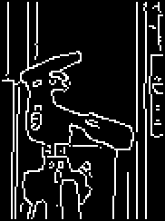
The call to rci_show differs from previous usage in assigning its result to rc_window. This will allow us to draw the lines we find on the display. The final line sets up the *RC_GRAPHIC scales and origin to facilitate this.
Since the boundslist of bin_edges is [83 173 67 188], its centre is close to column 128, row 128. So to get from row and column in the image to x and y, you can just subtract 128 from each of them. (Of course y will then run downwards again - reverse it if you wish.)
You should now be able to write Hough transform code that creates and fills a straight line accumulator array, using the data from bin_edges. It is not very complicated. You need to create an array with boundslist [0 99 0 99] and initialise it to zero. Then you will have a double outer for loop to scan the edge array. For each non-zero pixel encountered, the code will loop over theta, as in the examples above, but incrementing theta by 3.6° rather than by 10° on each step. For each theta, r will be found as before, but instead of drawing something, the code needs to add 1 to the appropriate element of the accumulator array. It will have to test for negative values of r, and ignore them.
If you want to try that, do so now. Rather than embedding more code in this teach file, the results you should get will be demonstrated using an efficient library program, *STRAIGHT_HOUGH:
    vars accumulator, rtheta, xc, yc;
    straight_hough(bin_edges, false, 100, 100, false, false,
        false, false, false, false) -> (accumulator, rtheta, xc, yc);
The <false> arguments just correspond to options that we do not need to use at the moment. The rtheta result will be described below, and xc and yc report the position in the array of the origin of (x, y) coordinates. The accumulator result is the accumulator array, which we can display as for an image:
rci_show(accumulator) -> ;
Although there are no axes in this display, they are laid out as for the earlier windows, except that theta now runs down the screen. The display may look like a rather murky view of a nebula, but a few bright dots are clear - particularly those at the top, where theta = 0°, and in the middle, where theta = 180°. These correspond to the strong vertical lines in the image, which get more votes by far than any other lines.
We can see more structure in the accumulator array if we compress the brightness scale for the higher values. One way to do this is to take the square root of all the accumulator bins before display. This sort of thing is very simple in Pop-11:
rci_show(mapdata(accumulator, sqrt)) -> ;
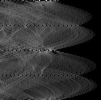
If there is still not a lot visible, try adjusting the brightness of your screen.
The shapes that now appear will be familiar from the earlier graphs. You can see how brighter points are visible where the curves for separate edge elements intersect.
Having got a filled accumulator array, the next thing to do is to locate the peaks in it. It is easy to write a program to find the location of the largest element of an array, or you can use array_peak from the *ARRAY_PEAKS library. This will tell you that the largest element of the accumulator array given by straight_hough is at column 39, row 0. You need to convert that into r and theta. This is not difficult, but in fact straight_hough helps by returning as its second result a Pop-11 procedure for doing the conversion.
This makes it simple to plot the line corresponding to the peak in question. We can use rt_draw_line to draw on the edge display, provided we move the coordinate system to have its origin at (xc, yc).
    rtheta(39, 0) -> (r, theta);        ;;; convert to r, theta
    rc_shift_frame_by(xc, yc);          ;;; shift coord origin
    XpwSetColor(rc_window, 'red') -> ;
    draw_rt_line(r, theta);
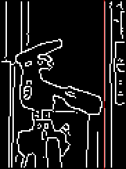
The long vertical line now marked in red is, not surprisingly, the one that received the most votes in the accumulator array. (The red line was drawn on the edge map display, so if that has got covered up, you will need to uncover it by removing or destroying windows. Don't forget that windows created by rci_image can be removed just by clicking on the image.)
Smaller peaks in the accumulator array correspond to shorter lines. By giving some more arguments to straight_hough, we can tell it to return a list of these peaks in descending order of number of votes. For details see the help file. The next chunk of code illustrates the results by plotting some of the most prominent lines on the original image, using a procedure provided in lib *STRAIGHT_HOUGH for finding the coordinates at which a line crosses the image boundary.
    ;;; get the list of accumulator peaks
    vars peaklist;
    straight_hough(bin_edges, false, 100, 100, false, false, false,
        false, 5, false) -> (accumulator, peaklist, xc, yc);

    rci_show(image) -> rc_window;
    rci_show_setcoords(image);      ;;; prepare to draw on image
    XpwSetColor(rc_window, 'red') -> ;

    vars peak, x0, y0, x1, y1;
    for peak in peaklist do
        hough_linepoints(peak, xc, yc, image) -> (x0, y0, x1, y1);
        rc_jumpto(x0, y0);
        rc_drawto(x1, y1);
    endfor;
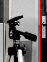
The strong vertical lines are naturally the ones detected. The penultimate argument to straight_hough is a threshold, determining how many votes are needed before a peak appears in the results (relative to the average number of votes in a bin). By reducing this threshold you can see more lines - ultimately the horizontal line in the middle is picked up, but you will also find that the edge elements start to interact to produce inaccurate or spurious lines.
You can restrict attention to near the tripod handle with a boundslist-type argument, and so detect the diagonal and horizontal lines in this region, with
    straight_hough(bin_edges, [120 160 130 150], 20, 20, false, false,
        false, false, 5, false) -> (accumulator, peaklist, xc, yc);
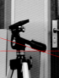
A 20 x 20 accumulator is appropriate because the small region means that line parameters are less precisely fixed by the data. Repeat the display code above to see the lines found. Since the Hough transform is a global method, in that it integrates information over the entire image or region that it is given, it is not surprising that we need a way of focussing attention if it is to give information about features of limited size.
In order to discuss the main principles, this teach file has skated over some quite important details.
One detail is the question of why it is safe to ignore negative r values returned by line_r. Going back to the original explanation of line parameters, a negative r means that after turning through theta, you walk backwards away from the origin. This is just equivalent to turning through an extra 180° and walking forwards - in other words a line with parameters (-r, theta) is identical to one with parameters (r, theta+180). If negative values of r were included in the parameter space, each line would get recorded twice. In fact, in an efficient implementation, theta only needs to run from 0 to 180°, and the negative r parameters are converted using -r -> r and theta + 180 -> theta before being recorded.
A second issue is how to detect peaks in the accumulator array. Finding local maxima (i.e. elements with values larger than those of their 8 neighbours) is the obvious thing to do. However, if the "true" parameters of a line happen to lie close to a boundary in the quantised parameter space, the votes will get spread over two or more bins, and looking at single bins may not reveal the peak. This can be helped to some extent by smoothing the accumulator array using convolution, before searching for peaks. In addition, one can sometimes do better than assuming that the peak position is at the centre of a bin - if an adjacent bin is large as well, it might be worth averaging their indices to estimate the peak position. The *STRAIGHT_HOUGH library incorporates these refinements in its peak detection - see the help file for details.
We have allowed each edge element in the bin_edges array the same number of votes. It seems reasonable that edge elements supported by a strong grey-level gradient should have more votes. It is easy to implement this: instead of incrementing the accumulator bins by 1 each time, you add in edge strength values depending on the size of the gradient for the current edge element. The straight_hough procedure implements this directly, and you can try it out easily by omitting the thresholding step used to binarise bin_edges. Alternatively, run the code in TEACH *STRAIGHT_HOUGH. You should find that the performance is somewhat improved. Using weighted votes this way fits in well with the idea of accumulation of evidence - strong edges provide more evidence. In fact, it is possible to relate the Hough transform to formal theories of inference, such as Bayesian theory.
Thresholding and edge weighting make use of the gradient magnitude, but can we also make use of the gradient direction? In fact, if we assume that the orientation of the edgelet at each pixel is known (e.g. it might be taken to be at right angle to the gradient direction), then we can simplify the Hough transform considerably. Each edge element then only votes for one bin in the accumulator, since theta is fixed by the edge orientation.
This has not been used here, for two reasons. First, the local gradient direction is rarely accurate enough to allow us to implement this scheme reliably as it stands - the information has to be used much more carefully. Second, the Hough transform presented here illustrated the general method a good deal better, and is more amenable to generalisation.
I mentioned earlier that the choice of quantisation is a big problem. One way round that is to start by doing a Hough transform with a very coarse quantisation of parameter space. You then subdivide those bins with lots of votes, and do another transform into just these parts of parameter space, with the finer quantisation. The process is repeated until the bins are as small as necessary.
This method has been used successfully, but may be delicate: a lot of small peaks in one part of parameter space will stop you seeing a single larger peak in another part.
The Hough transform is not restricted to detecting straight lines, though that is a common use. Other geometrical shapes that can be described with a few parameters are also well suited to it.
For example, a circle is specified with three numbers: the X and Y coordinates of its centre, and R, its radius. To find circles using a Hough transform, you need a three-dimensional accumulator array. Each edge element votes for all the circles that it could lie on, and the 3-D array is searched for peaks that give circle positions and radii. If you happen to know the radius in advance, you only need a 2-D accumulator - you should not find it difficult to implement this yourself if you want to experiment.
More complicated shapes can be found - a general ellipse, for example, needs a 5-D parameter space. Hough transforms have also been used for finding vanishing points - the points to which the images of parallel sets of lines appear to converge.
Finally, the method can be generalised to detecting any shape that can be represented by a finite number of line segments, but which may appear at any orientation, scale and position in the image. The parameter space is, in general, 4-dimensional (2 for position, 1 for orientation, 1 for scale), and it helps if straight line segments are extracted from the image first. This generalised Hough transform is described in several of the books mentioned in TEACH *VISION, for example Ballard & Brown's 'Computer Vision'.
You should now have a clear grasp of how the Hough transform for straight line detection works, and you should have some idea of how it can be generalised.
Here are links to:
Copyright University of Sussex 1994. All rights reserved.