Recently, Orr [126] analyzed several prominent three dimensional scene analysis systems, including the IMAGINE I system described here, and concluded that five generic functions provided the geometric reasoning needed for most computer vision tasks. The functions were:
At the time of the research undertaken here, two of the best approaches to representing position estimates were based on either an explicit complete position, perhaps with some error estimates (i.e. from a least-squared error technique, such as Faugeras and Hebert [63]) or by parameter ranges, linked to algebraic inequality constraints over the parameters (as in the ACRONYM system [42]).
The first approach integrated a set of uniform data (e.g. model-to-data vector pairings) to give a single-valued estimate, but at some computational cost. On the other hand, ACRONYM's advantage was that it could easily integrate new evidence by adding new constraints, the range of possible values was made explicit and inconsistency was detectable when parameter ranges became non-existent. Its disadvantage was that the current estimate for a parameter was implicit in the set of constraints and could only be obtained explicitly by substantial algebraic constraint manipulation of non-linear inequalities, which result only in a range of values with no measure of "best".
More recent work by Durrant-Whyte [57] represented position estimates statistically, computing the transformations of positions by a composition technique. This has the advantage of propagating uncertainties concisely and gives a "best" estimate, but does not easily provide the means to determine when inconsistency occurs (other than low probability). Further, approximations are needed when the reference frame transformations themselves involve uncertainty, or when uncertainty is other than statistical (e.g. a degree-of-freedom about a joint axis).
The techniques used in IMAGINE I are now described, and related to the five function primitives described above.
Each individual parameter estimate is expected to have some error, so it is represented by a range of values. (The initial size of the range was based on experience with parameter estimation.) An object's position is then represented by a six dimensional parameter volume, within which the true parameter vector should lie. Thus, the position representation is a simplified, explicit version of that used by ACRONYM (but less precise, because constraint boundaries are now planes perpendicular to the coordinate axes). This leads to more efficient use, while still representing error ranges and detecting inconsistency.
Integrating parameter estimates (i.e. MERGE) is done by intersecting the individual parameter volumes. All the six dimensional parameter volumes are "rectangular solids" with all "faces" parallel, so that the intersection is easily calculated and results in a similar solid. Because the true value is contained in each individual volume, it must also lie in the intersection. The effect of multiple estimates is to refine the tolerance zone by progressively intersecting off portions of the parameter volume, while still tolerating errors. If a final single estimate is needed, the average of each pair of limits is used.
As described so far, the transformation of coordinate reference systems (TRANSFORM) has been done by multiplication of the homogeneous coordinate matrices representing the transforms. Since we are now using a parameter estimate range, the transformation computation must be modified. In the most general case, each transformation would have its own range, but, as implemented here, only the transformation from the camera coordinate system to the object global reference frame is allowed statistical variations. (Although, transformations may have parameterized degrees-of-freedom - see Chapter 7.) These variations propagate through the calculation of the global or image locations for any feature specified in any level of reference frame. The variation affects two calculations:
The technique used for both of these problems is similar, and is only an approximation to a complete solution:
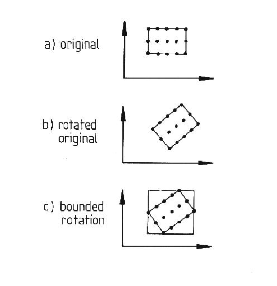
This process is illustrated in Figure 9.1. In part (a), a two dimensional parameter range with the subset of points is designated. In part (b), the original range is rotated to a new range, and part (c) shows the parameter bounds for the new range.
The figure illustrates one problem with the method - parameter bounds are aligned parallel with the coordinate axes, so that the parameter volume (actually six dimensional) increases with each transformation. A second problem is that the rotation parameter space is not rigid in this coordinate system, so that the shape of the parameter space can change greatly. If it expands in a direction not parallel with a coordinate axis, the combination of the first problem with this one can result in a greatly expanded parameter space. Further, the transformation is not unique, as zero slant allows any tilt, so any transformations that include this can grow quickly.
One general problem with the method is that consistent data does not vary the parameter bounds much, so that intersecting several estimates does not always tighten the bounding greatly. Hence, there is still a problem with getting a "best" estimate from the range. Another problem with the general case is that each model variable increases the dimensionality of the parameter space, requiring increased computation and compounding bounding problems.
The conclusion is that this simplified method of representing and manipulating parameter estimates is not adequate, which led to the work by Fisher and Orr [74] described here.
The INVERSE function occurs in two forms. Inverting an exact transformation (represented by a homogeneous coordinate matrix) is simply matrix inversion. Inverting an estimate range is given by bounding the inversions of a subset of the original range (similar to TRANSFORM).
The PREDICT function uses either an exact transformation from the model or the mean value of a data-derived parameter range to predict either three dimensional vector directions, three dimensional points or two dimensional points (by projection of the three dimensional points).
The LOCATE function is specific to the data and model feature pairings, and is described in more detail in the next two sections.