Network Based Geometric Reasoning

Position errors result from two causes - errors in the input data and deficiencies in the position estimation algorithms. To help remove the second source, Fisher and Orr [74] developed a network technique based on the algebraic method used in ACRONYM. The technique implements the constraint relationships as a value-passing network that results in tighter bounds and improved efficiency. Moreover, we observed that the forms of the algebraic constraints tended to be few and repeated often, and hence standard subnetwork modules could be developed, with instances allocated as new position constraints were identified. Examples of these network modules are: "a model vector is transformed to a data vector" and "a data point must lie near a transformed model point".

There are three aspects to the new network-based geometric reasoner:

1. specifying the geometric problem as algebraic constraints,
2. evaluating the constraints in a value-passing network and
3. partitioning the network into prototypical modules.

These are now described in more detail.

The key data type is the position, which represents the relative spatial relationship between two features (e.g. world-to-camera, camera-to-model, or model-to-subcomponent). A position consists of a 3-vector representing relative translation and a unit 4-vector quaternion representing relative orientation (of the form $(cos(\theta / 2), sin(\theta / 2)\vec{w})$ for a rotation of $\theta$ about the axis $\vec{w}$).

The key geometric relationships concern relative position and have two forms: exact and partially constrained. An example of an exact form is: let object A be at global position $(\vec{r}_A,\vec{t}_A)$, (translation $\vec{t}_A$ and rotation $\vec{r}_A$) and object B be at $(\vec{r}_{AB},\vec{t}_{AB})$ relative to A. Then, the global position of B is:

$$(r_{AB}*r_A,r_{AB}*t_A*r_{AB}' + t_{AB})$$

where $*$ is the quaternion multiplication operator:

$(q_0,q_1,q_2,q_3)*(p_0,p_1,p_2,p_3)$
$= (q_0p_0 - q_1p_1 - q_2p_2 - q_3p_3, q_2p_3 - q_3p_2 + q_0p_1 + q_1p_0,$ $q_3p_1 - q_1p_3 + q_0p_2 + q_2p_0, q_1p_2 - q_2p_1 + q_0p_3 + q_3p_0)$

and the quaternion inverse operator " $'$ " is:

$$(r_0,r_1,r_2,r_3)' = (r_0,-r_1,-r_2,-r_3)$$

A partially constrained position is given by an inequality constraint, such as:

$$t_{Az} \geq 50$$

This means that the $z$ component of A's global position is at least 50. Such a constraint might arise from some a priori scene knowledge, or observing a fragment of a surface.

Other relationships concern vectors or points linked by a common transformation, as in $T\vec{v}_1 = \vec{v}_2$, or the proximity of points or vectors:

$$\mid \vec{p}_1 - \vec{p}_2 \vert < \epsilon$$

Instances of these constraints are generated as recognition proceeds. Then, with a set of constraints, it is possible to estimate the values of the constrained quantities (e.g. object position) from the known model, the data values and their relationships. Alternatively, it may be possible to determine that the set of constraints is inconsistent (i.e. the set of constraints has no solution), and then the hypothesis is rejected.

A key complication is that each data measurement may have some error or uncertainty, and hence the estimated values may also have these. Alternatively, a variable may be only partially constrained in the model or a priori scene information. Hence, each numerical quantity is represented by an interval [7]. Then, following ACRONYM with some extensions, all constraints are represented as inequalities, providing either upper or lower bounds on all quantities.

We now look at how the constraints are evaluated.

ACRONYM used a symbolic algebra technique to estimate upper (SUP) and lower (INF) bounds on all quantities. When bounds cross, i.e. $SUP(x) < INF(x)$, then inconsistency was declared and the hypothesis rejected. This symbolic algebra method was slow and did not always give tight bounds.

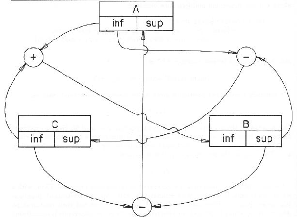
The basis of the network approach is the propagation of updated bounds, through functional units linked according to the algebraic problem specification. A simple example is based on the inequality:

$$A \leq B - C$$

By the SUP/INF calculus ([33,151,42]), the upper bound of $A$ is constrained by:

$$SUP(A) \leq SUP(B) - INF(C)$$

as are the lower bounds of B and C:

$$INF(B) \geq INF(A) + INF(C)$$

$$SUP(C) \leq SUP(B) - INF(A)$$

Thus, one can use the value of $SUP(B) - INF(C)$ as an estimated upper bound for A, etc. These relationships are used to create the network for this single inequality, which is shown in Figure 9.9. As new bounds on (for example) B are computed, perhaps from other relationships, they propagate through the network to help compute new bounds on A and C.

Figure 9.9: Small Constraint Network

There are two advantages to the network structure. First, because values propagate, local improvements in estimates propagate to help constrain other values elsewhere. Hence, even though we still have rectangular interval parameter space bounds, the constraints are non-rectangular and thus can link changes in one variable to others. Even for just local problems, continued propagation until convergence produces better results than the symbolic methods of ACRONYM. Second, these networks have a natural wide-scale parallel structure (e.g. 1000+) that might eventually lead to extremely fast network evaluation in VLSI (e.g. 10-100 microseconds). One disadvantage of the network approach is that standard bounding relationships must be pre-computed as the network is compiled, whereas the symbolic approach can be opportunistic when a fortuitous set of constraints is encountered.

For a given problem, the networks can be complicated, particularly since there may be both exact and heuristic bounding relationships. For example, the network expressing the reference frame transformation between three positions contains about 2000 function nodes (of types "+", "-", "*", "/", "sqrt", "max", "greaterthan", "if" etc.). The evaluation of a network is fast, even in serial, because small changes are truncated to prevent trivial propagations, unlike other constraint propagation approaches (see [53]). Convergence is guaranteed (or inconsistency detected) because bounds can only tighten (or cross), since only sufficiently large changes are propagated.

The creation of the networks is time-consuming, requiring a symbolic analysis of the algebraic inequalities. Fortunately, there is a natural modular structure arising from the types of problems encountered during scene analysis, where most geometric constraints are of a few common types. Hence, it is possible to pre-compile network modules for each relationship, and merely allocate a new instance of the module into the network as scene analysis proceeds. To date, we have identified and implemented network modules for:

SS

- two scalars are close in value

PP

- two points are close in location

VV

- two vectors point in nearly the same direction

TP

- a transformation links a pair of points

TV

- a transformation links a pair of vectors

TV2

- a transformation links two pairs of vectors

TT

- a transformation links from one position to a second by a third position

P2V

- a vector can be defined by two points

QWT

- a quaternion is equivalent to an axis of rotation and an angle

One important feature of these modules is that they are bi-directional, in that each variable partially constrains all other related variables. Hence, this method is usable for expressing partial constraints (such as "the object is above the table" or $Z \geq 0$). The constraints on other related variables can then help fully constrain unbound or partially constrained variables.

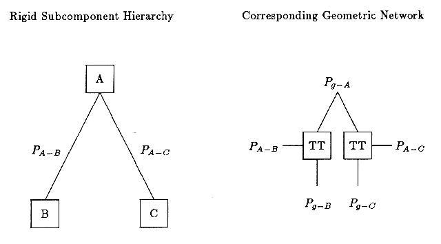
We now include a simple and a complicated example of network use. Suppose subcomponents B and C are rigidly connected to form object A. With the estimated positions of the subcomponents in the global coordinate system, $P_{g-B}$ and $P_{g-C}$, and the transformations between the object and local coordinate systems, $P_{A-B}$ and $P_{A-C}$, then these can be used to estimate the global object position, $P_{g-A}$, by using two instances of the "TT" module listed above. Figure 9.10 shows this network. Notice that each subcomponent gives an independent estimate of $P_{g-A}$, so that the network keeps the tightest bounds on each component of the position. Any tighter resulting bounds then propagate back through the modules to refine the subcomponent position estimates.

Figure 9.10: A Simple Geometric Reasoning Network

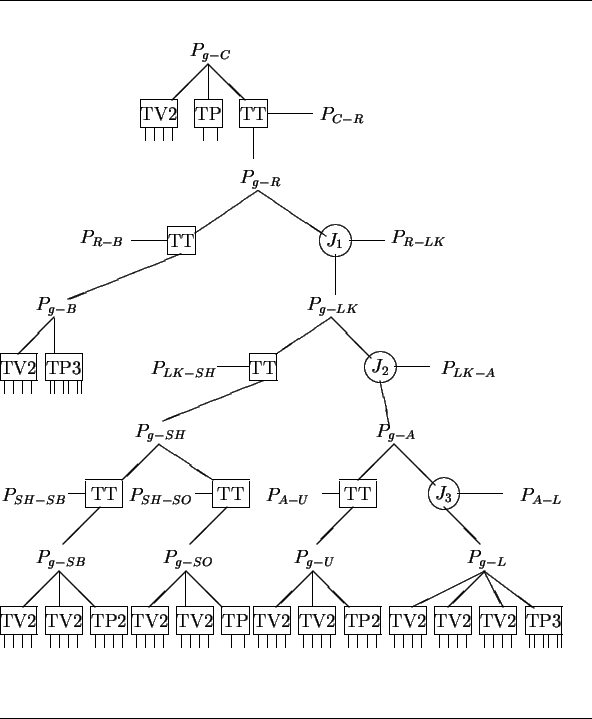
Figure 9.11 shows the full network generated for analyzing the robot in the test scene. As before, the boxes represent transformations, but there are more types used here. The "TP$n$" boxes stand for $n$ instances of a "TP" module. The circular "$J_n$" boxes represent three identical instances of subnetworks allocated for transformations involving joint angles, which are omitted to simplify the diagram (each contains 7 network modules). The relative positions of objects are given by the $P$ structures, such as $P_{g-R}$, which represents the position of the robot in the global reference frame. These are linked by the various transformations. Links to model or data vectors or points are represented by the unconnected segments exiting from some boxes.

Figure 9.11: Robot Scene Geometric Reasoning Network

The top position $P_{g-C}$ is the position of the camera in the global coordinate system, and the subnetwork to the left and below relates features in the camera frame to corresponding ones in the global coordinate system. Below that is the position $P_{g-R}$ of the robot in the global coordinate system and the position $P_{C-R}$ of the robot in the camera coordinate system, all linked by a TT position transformation module. Next, to the bottom left is the subnetwork for the cylindrical robot body $P_{g-B}$. The "$J_1$" node connects the robot position to the rest ("link") on the right, whose position is $P_{g-LK}$. Its left subcomponent is the rigid shoulder ASSEMBLY (SH) with its subcomponents, the shoulder body (SB) and the small shoulder patch (SO). To the right, the "$J_2$" node connects to the "armasm" ASSEMBLY (A), linking the upper arm (U) to the lower arm (L), again via another joint angle ("$J_3$"). At the bottom are the modules that link model vectors and points to observed surface normals, cylindrical axis vectors, and central points, etc. Altogether, there are 61 network modules containing about 96,000 function nodes.

The network structure closely resembles the model subcomponent hierarchy, and only the bottom level is data-dependent. There, new nodes are added whenever new model-to-data pairings are made, producing new constraints on feature positions.

Evaluating the complete network from the raw data requires about 1,000,000 node evaluations in 800 "clock-periods" (thus implying over 1000-way parallelism). Given the simplicity of operations in a node evaluation, a future machine should be able to support easily a 1 microsecond cycle time. This suggests that an approximate answer to this complicated problem could be achieved in about 1 millisecond.

As the tolerances on the data errors propagate through the network modules, they do not always produce tight result intervals, though some interval reduction is achieved by integrating separate estimates. For example, if each orientation component of a random position $P_{a-b}$ has interval width (i.e. error) $\delta$ and each orientation component of a random position $P_{b-c}$ has interval width $\epsilon$, then each component of the resulting position $P_{a-c} = P_{a-b} * P_{b-c}$ has interval width:

$$\frac{16(\delta + \epsilon)}{3\pi}$$

However, this interval width is less or non-existent for most of the actual rigid transformations used here.

Because the resulting intervals are not tight, confidence that the mean interval value is the best estimate is reduced, though the bounds are correct and the mean interval values provide useful position estimates. To tighten estimates, a post-processing phase iteratively shrinks the bounds on a selected interval and lets the new bounds propagate through the network. For the robot example, this required an additional 12,000 cycles, implying a total solution time of about 13 milliseconds on our hypothetical parallel machine.

Using the new geometric reasoning network, the numerical results for the whole robot in the test scene are summarized in Table 9.10. Here, the values are given in the global reference frame rather than in the camera reference frame.

Table 9.10: Measured And Estimated Spatial Parameters

PARAMETER	MEASURED	ESTIMATED
X	488 (cm)	487 (cm)
Y	89 (cm)	87 (cm)
Z	554 (cm)	550 (cm)
Rotation	0.0 (rad)	0.038 (rad)
Slant	0.793 (rad)	0.702(rad)
Tilt	3.14 (rad)	2.97 (rad)
Joint 1	2.24 (rad)	2.21 (rad)
Joint 2	2.82 (rad)	2.88 (rad)
Joint 3	4.94 (rad)	4.57 (rad)

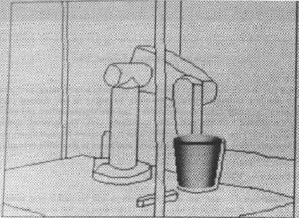
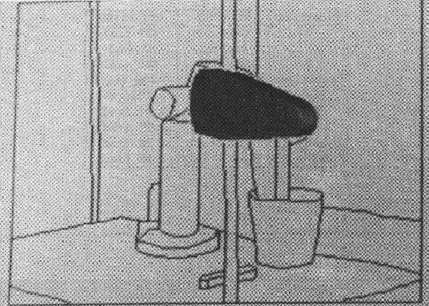
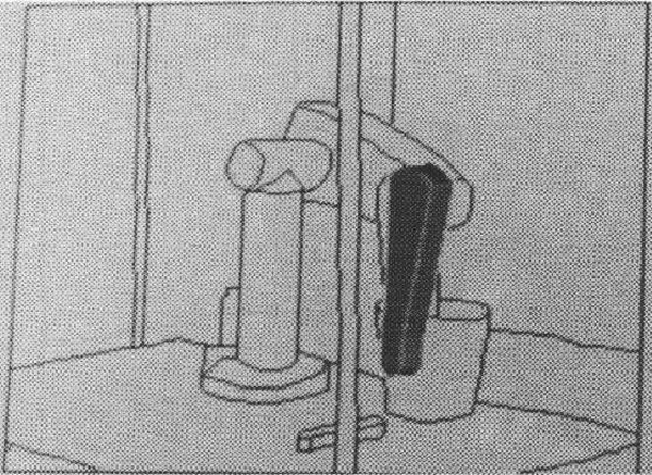
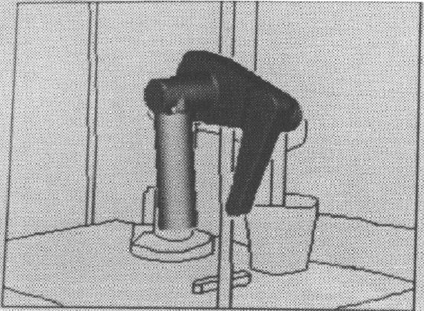
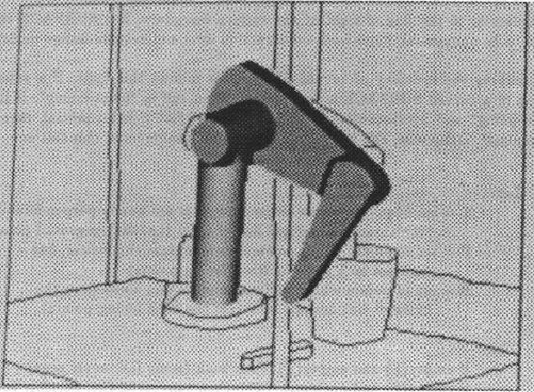
The results of the position estimation can been seen more clearly if we look at some figures showing the estimated object positions overlaying the original scene. Figure 9.12 shows the estimated position of the trash can is nearly correct. The robot upper arm (Figure 9.13) and lower arm (Figure 9.14) are also close. When we join these two to form the armasm ASSEMBLY (Figure 1.10), the results are still reasonable, but by the time we get to the whole robot (Figure 9.15), the accumulated errors in the position and joint angle estimates cause the predicted position of the gripper to drift somewhat from the true position (when using the single pass at network convergence). The iterative bounds tightening procedure described above then produces the slightly better result shown in Figure 1.11. Note, however, that both network methods produced improved position results over that of the original IMAGINE I method, which is shown in Figure 9.16.

Figure 9.12: Recognized Trash Can

Figure 9.13: Recognized Upper Arm

Figure 9.14: Recognized Lower Arm

Figure 9.15: Recognized Complete Robot Using One-Pass Network Method

Figure 9.16: Original IMAGINE I Recognized Complete Robot

Though research on the efficient use of these networks is continuing, problems overcome by the new technique include the weak bounding of transformed parameter estimates and partially constrained variables, and the representation and use of constraints not aligned with the parameter coordinate axes. The network also has the potential for large scale parallel evaluation. This is important because about one-third of the processing time in these scene analyses was spent in geometric reasoning.