


Next:Zoom-Lens
Camera CalibrationUp:Zoom-lens
Camera CalibrationPrevious:Camera
Calibration Problem
Neurocalibration
In [1] we proposed a MLFN that
not only learns perspective projection mapping of a camera, but also can
specify the calibration parameters. The neurocalibration net has a topology
of 4-4-3 with linear hidden and output neurons (see the central net
in Fig. 1). The weight matrix of the
hidden layer is denoted by V, and it is assumed
to correspond to the extrinsic parameters. The weight matrix of the output
layer is denoted W and it corresponds to the
intrinsic parameters, or matrix A. For any
input pattern Mi, the network output, (oik,
k=1,2,3), represents the 2D pixel homogeneous coordinates. In terms
of the network parameters, the error in (1)
can be expressed as [1]
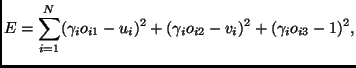 |
(2) |
where  is a parameter attached to each input point, and takes care of the fact
P is defined up to a scale factor that may
be different from one point to another. One can look at
as the slope of the linear activation function of the output neurons. The
weights of the network Wkj and Vlj
are initialized at random values in the range -1:1, while all the different
are initially set to 1. The network weights Wkj,
Vlj and
are updated according to the gradient descent rule applied to Eq.(2)
[1]. For ease of network learning,
the input and desired patterns of the network are normalized by s1
and s2, respectively. After training the network, the
projection matrix P can be shown to be
[1]
is a parameter attached to each input point, and takes care of the fact
P is defined up to a scale factor that may
be different from one point to another. One can look at
as the slope of the linear activation function of the output neurons. The
weights of the network Wkj and Vlj
are initialized at random values in the range -1:1, while all the different
are initially set to 1. The network weights Wkj,
Vlj and
are updated according to the gradient descent rule applied to Eq.(2)
[1]. For ease of network learning,
the input and desired patterns of the network are normalized by s1
and s2, respectively. After training the network, the
projection matrix P can be shown to be
[1]
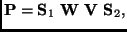 |
(3) |
where
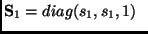 and and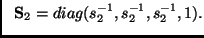 |
|
In order to go beyond just obtaining the matrix P,
the camera parameters are also obtained by mapping each network weight
to one camera parameter. This can be done by enforcing the orthogonality
constraints on R during network learning. The
constraints are represented as additional terms added to the error criterion
to be minimized. The new error measure will be
 |
(4) |
where  is the same in (2) and
  is a sum of six error terms [1]
that ensure the weights matrix V to be a rotation
matrix. The positive weighting factor,
is a sum of six error terms [1]
that ensure the weights matrix V to be a rotation
matrix. The positive weighting factor,  ,
increases slowly as learning proceeds.
,
increases slowly as learning proceeds.
The network is trained by the traditional Backpropagation algorithm,
however, speedup can be achieved by applying the conjugate gradient method
during some periods of the training process. Switching between conjugate
gradient and gradient descent can be done automatically (for details, see
[5]).
Our extensive simulations and tests on practical images [1]
yielded very low calibration error and have shown that this neurocalibration
approach has the following features:
-
it relaxes the requirement of a good initial starting point, which is common
to other non-linear optimization techniques (e.g., Levenberg-Marquardt
algorithm). These techniques often fail without this condition. In all
the experiments conducted, the network has converged starting from random
initial weights without sacrificing the calibration accuracy.
-
experiments have shown very small sensitivity of the network learning to
network parameters, e.g., learning constants.
-
the orthogonality constraints on the rotation matrix are satisfied in the
obtained parameters without extra optimization steps [12].
-
it is simple; the reader can easily reproduce our code.
-
it is interesting to note that the above network can be easily modified
to calibrate some other camera models, in particular, for calibrating linear
pushbroom cameras [2] which may
be thought of as a hybrid of perspective projection in one imaging direction
and orthographic projection in the other direction.
These features motivated us to use the neurocalibration net for the global
optimization step of zoom-lens calibration.
Next:Zoom-Lens
Camera CalibrationUp:Zoom-lens
Camera CalibrationPrevious:Camera
Calibration Problem
Moumen T. Ahmed 2001-06-27