Rhodri H Davies, Neil A Thacker and Chris J Taylor
These notes contain an overview of the B-fitting method proposed by Thacker et al [1]. The method is a model-selection criteria that explicitly calculates the generalisation ability of the model.
MATLAB code that demonstrates B-Fitting polynomials to some 1D data can be found at:
http://www.isbe.man.ac.uk/![]() rhd/code/Bhatt/.
rhd/code/Bhatt/.
The `README.m' file contains instructions on how to run the demos.
Model-fitting involves estimating (i.e. modelling) the process that generated a set of data. We usually use a subset of the entire dataset (the training set) to estimate the model.
We must find a suitable compromise for the model's complexity, this is often referred to as the principle of parsimony. If the model is too complex, it will capture the errors in the training set and be unable to generalise to unseen data. If it is too simple, it will not be a sufficient estimate of the intrinsic process that created the data.
Ideally, the model should be chosen so that it encodes the meaningful, systematic aspects of the data and discards the unstructured portion.
The Chi-squared metric is a `goodness of fit' measure that is often used to assess the suitability of a given model. It looks like:
![]()
where ![]() is a set of parameters,
is a set of parameters, ![]() is the true value at point i,
is the true value at point i, ![]() is the predicted value at that point and
is the predicted value at that point and ![]() is the data measurement accuracy (the probable variance of the error).
is the data measurement accuracy (the probable variance of the error).
The drawback of using the ![]() -metric is that it places no restriction on the complexity of the model, making it prone to overfitting on the training set.
-metric is that it places no restriction on the complexity of the model, making it prone to overfitting on the training set.
Many methods have been proposed to prevent overfitting by penalising model complexity (e.g. Aikake's information criterion - AIC ). These typically take the form:
Goodness of fit = Training error + Complexity
It is not, however, entirley clear how to select the complexity term.
B-Fitting is a method that gives an unbiased measure of the generalisation ability of a model.
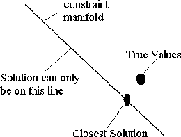
Consider a least-squares fit. It attempts to find the model that minimises the squared-distances between ![]() and
and ![]() . See the diagram in figure 1 - here, the solution is constrained to lie on a manifold (illustrated as a line). A least-squares fit will select the point on the manifold that is closest to the correct solution.
. See the diagram in figure 1 - here, the solution is constrained to lie on a manifold (illustrated as a line). A least-squares fit will select the point on the manifold that is closest to the correct solution.

Figure 1: A least squares fit in hyperspace
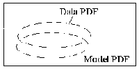
B-Fitting, however, not only attempts to find the shortest distance but also considers the stability of the model. A set of solutions and probable errors can be described by a multivariate probability distribution function (pdf). We already have this information for the data (from the training set) and assuming we also have the information of the model, B-fitting states that the optimal solution is when the two pdf's have maximum overlap. See Figure 3 - again, the solution must lie along the constraint manifold but this time we attempt to overlap the pdfs as much as possible.

Figure 2: B-fitting in a hyperspace

Figure 3: The optimal solution
B-fitting makes use of the Bhattacharya metric to measure the similarity (amount of overlap) of two pdf's.
The Bhattacharya metric has many desirable statistical properties [2] that make it a suitable measure of the divergence of two pdfs. The 1D analytical Bhattacharya measure for a Gaussian distribution is:
where ![]() is the distance between the data and the estimate (made by the model),
is the distance between the data and the estimate (made by the model), ![]() is the (error) variance of the data pdf and
is the (error) variance of the data pdf and ![]() is the probable variance of the model pdf.
is the probable variance of the model pdf.
We will now consider how we can estimate the error on the model.
![]()
where ![]() .
.
For the n-d case, if we assume the errors are normally distributed and independent, we can propagate the errors through the model with:
![]()
where y=f(x).