Construction of Spherical Codes

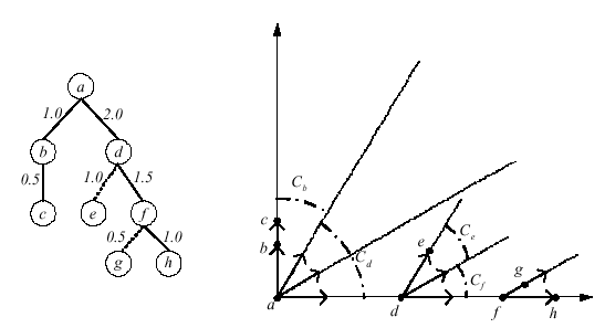
To embed our metric trees into Euclidean spaces of fixed dimension, we introduce the concept of spherical codes. Such codes, in turn, will allow us to directly compare two embeddings. The embedding framework is best illustrated through an example, in which a weighted tree is embedded into ${\mathbb{R}}^2$, as shown in Figure 4. To ease visualization, we will limit the discussion to the first quadrant. The weighted tree contains 4 paths $\left <a,b,c\right >$, $\left <a,d,f,h\right >$, $\left <d,e\right >$, and $\left < f,g\right >$ in its caterpillar decomposition. In the embedding, the root is assigned to the origin. Next, we seek a set of $4$ vectors, one for each path in the caterpillar decomposition, such that their inner products are minimized, i.e., their endpoints are maximally apart. These vectors define the general directions in which the vertices on each path in the caterpillar decomposition will be embedded.

Figure 4: An edge weighted tree and its spherical code in 2D. The Cartesian coordinates of the vertices are: $a=(0,0)$, $b=(0,1.0)$, $c=(0,1.5)$, $d=(2.0,0)$, $e=(2.5,0.87)$, $f=(3.5,0)$, $g=(3.93,0.25)$, and $h=(4.5,0)$.

Three of the four vectors will be used by the caterpillar paths belonging to the subtree rooted at vertex $d$, and one vector will be used by the path belonging to the subtree rooted at vertex $b$. This effectively subdivides the first quadrant into two cones, $C_b$ and $C_d$. The volume of these cones is a function of the number of caterpillar paths belonging to the subtrees rooted at $b$ and $d$. The cone $C_d$, in turn, will be divided into two smaller cones, $C_e$ and $C_f$, corresponding to the subtrees rooted at $e$ and $f$, respectively. The extreme rays of sub-cones $C_b$, $C_e$, and $C_f$ will correspond to the 4 directions defining the embedding. Finally, to complete the embedding, we translate the sub-cones away from the origin along their directional rays to positions defined by the path lengths in the tree. For example, to embed point $b$, we will move along the extremal ray of $C_b$ and will embed $b$ at $(0,1.0)$. Similarly, the sub-cone $C_d$ will be translated along the other extremal ray, embedding $d$ at $(2.0,0)$. In $d$-dimensional Euclidean space ${\mathbb{R}}^d$, computing the embedding $f:{\cal A}\rightarrow {\cal B}$ under $\vert\vert.\vert\vert _2$ is more involved. Let $L$ denote the number of paths in the caterpillar decomposition. The embedding procedure defines $L$ vectors in ${\mathbb{R}}^d$ that have a large angle with respect to each other on the surface of a hypersphere $S_d$ of radius $r$. These vectors are chosen in such a way that any two of their endpoints on the surface $\sum_d$ are at least spherical distance 2 from each other. We will refer to such vectors as well-separated. Consider the set of hyperplanes $H_i = ( 0, 2, 4, \ldots, 2i)$, and let $\sum_d(i) = H_i \cap \sum_d$. Since each of the $\sum_d(i)$ are hypercircles, i.e., surfaces of spheres in dimension $d-1$, we can recursively construct well-separated vectors on each hypercircle $\sum_d(i)$. Our construction stops when the sphere becomes a circle and the surface becomes a point in 2 dimensions. It is known that taking $r$ to be $O (dL^{1/{d-1}})$, and the minimum angle between two vectors to be $2/r$ provides us with $L$ well-separated vectors [6]. In Figure 4, we have 4 such vectors emanating from the origin. Now that the embedding directions have been established, we can proceed with the embedding of the vertices. The embedding procedure starts from the root (always embedded at the origin) and embeds vertices following the embedding of their parents. For each vertex in the metric tree ${\mathfrak{T}}$, we associate with every subtree ${\mathfrak{T}}_v$ a set of vectors $C_v$, such that the number of vectors in $C_v$ equals the number of paths in the caterpillar decomposition of ${\mathfrak{T}}_v$. Initially, the root has the entire set of $L$ vectors. Consider a subtree rooted at vertex $v$, and let us assume that vertex $v$ has $k$ children, $v_1,\ldots,v_k$. We partition the set of vectors into $k$ subsets, such that the number of vectors in each subset, $S_v$, equals the number of leaves in ${\mathfrak{T}}_v$. We then embed the vertex $v_l$ ($1 \le l \le k$) at the position $f(v) + w_l*x_l$, where $w_l$ is the length of the edge $(v, v_l)$ and $x_l$ is some vector in $C_{v}$. We recursively repeat the same process for each subtree rooted at every child of $v$, and stop when there are no more subtrees to consider.