Constrained reverse engineering

Parts have standard feature relationships

One of the cornerstones of the recent research in our laboratory has been constrained recovery of 3D shapes from 3D point cloud data. There has been much previous research on curved surface shape estimation, based either on the Euclidean distance [6] or variants of the algebraic distance [22]. Given the shape bias arising from the algebraic distance, researchers have also developed a general quadric surface extension to the algebraic distance using a gradient based weighting [52] or a shape specific approximation [31]. These fitting approaches were for single surfaces. In our case, we have used a constrained algebraic distance approach that applies shape specific constraints on all of the individual surfaces. Within the same framework, we also simultaneously apply constraints that encode standard feature relationships such as alignment of surfaces, colinearity of features, etc. This constrained reverse engineering technique has been applied to both industrial parts and architectural scenes.

Figure 2: Constrained freeform surface recovery. Left) Object. Right) constrained planar and mesh surfaces.

The key issue is how to incorporate shape and design constraints into shape fitting of 3D data. Our current approach is to formulate shape fitting as constrained least-squares problem. If:

• $\vec{p}$ specifies the parameter vector for feature shapes and positions
• ${\cal H}$ is the least squares shape error matrix
• $C_i(\vec{p})$ are constraints over the parameters
• $\lambda_i$ are penalty costs

and then minimize:

$$\vec{p}^T {\cal H} \vec{p} + \sum_i \lambda_i C_i(\vec{p})$$

The first term is a least squares fitting term that ensures that model surfaces lie close to the image data. The second term encodes the penalties for constraint violations. The linear least squares error term can also be a non-linear Euclidean distance (or other) error term. Minimizing this error is generally a non-convex problem, so we initialize $\vec{p}$ to be the standard least-square solution and $\lambda_i=0$ and then apply numerical optimization methods. We then incrementally enforce the constraints by increasing penalty costs $\lambda_i$ and re-minimizing until the constraints are satisfied to the desired tolerances. The gradual increase ensures that the solution stays near the least-square solution and also helps avoid local minima. Experiments show that solutions initialized from different randomly perturbed starting points converge to a small cluster of nearby solutions.

While we have only experimented with constraint functions $C()$ that use the square of the error in the constraint, one could also use a gated function that produces zero error if the constrained relationship is within a given tolerance. If this form were used, our gradient based optimization method would need to be modified as there is a discontinuity at the tolerance point. One possible approach is to use evolutionary methods mentioned in Section 6. Then the constraint can be simply ignored in the evaluation function if the specified tolerance is satisfied.

We have applied this approach to engineering parts modeled by planar and quadric surfaces [55,56]. The surfaces are extracted from range images or point clouds by a segmentation process based on 1) shape discontinuity detection, 2) boundary constrained noise smoothing, 3) principal curvature based local shape classification and finally 4) quadric surface fitting. A recent comparison in [26] concluded that in many ways our single image planar surface segmentation algorithm had the best performance among current algorithms.

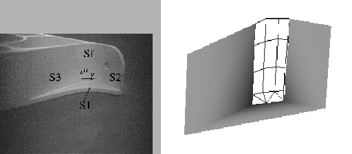
The part shown in Figure 1 has constraints between planar, cylindrical and conical surfaces. Seven shape relation constraints were applied. All constraints can be satisfied while still maintaining close surface fitting. Applying the constraints also improves shape parameter recovery. For example, the top cylindrical surface has the true radius of 60 mm. Initial least-square quadric fitting estimated an elliptic cylinder radius of 33-46 mm. Adding the relationship constraints resulted in a circular cylinder radius estimate of 59.54 mm.

One can also apply the approach [57] to enforcing inter-surface boundary constraints between freeform and quadric surfaces, while also trying to minimize surface fitting error. This differs from the pure constrained freeform surface case [30] and the pure quadric surface case [55,56]. We also considered constraints between non-adjacent surfaces as well as connectivity constraints. We satisfied the constraints effectively exactly using a numerical optimization process instead of an equation-solving approach [44], using the data projection method of [33]. One application is ensuring that the freeform surface is tangential or orthogonal to a planar surface at their common boundary. Figure 2 shows three mutually orthogonal planar surfaces plus a B-spline surface tangential to two of the planes and orthogonal to the third.

Figure 3: Constrained recovery of an architectural scene. Top) Original VRML object with surface ripples most easily seen at lower left. Bottom) Flattened and constrained surfaces with fewer artifacts.

More recently, we applied the constrained shape fitting method to architectural scenes [9]. The concepts are similar to the industrial part case as many standard architectural relationships are present, such as near perpendicularity of walls and floors, coplanarity of floors inside and outside rooms, etc. Additionally, as we know that we are recovering a building with large planar surfaces, we can recover a better model by enforcing surface flatness by displacing triangle vertices onto the nearest plane. Figure 3 shows some ripples near the lower windows in the original triangulation that have been flattened. The data for this example was acquired by an expensive range sensor, but some of our other examples [9] have used sparse 3D triangulated point sets obtained from structure-and-motion recovery from video sequences. Due to the sparseness of the 3D triangulated data features, we needed a different segmentation process to assign vertices to planar surface patches. After that, constrained surface adjustment and fitting proceeded in the same way as the part shape recovery. The use of structure-and-motion data would probably not be so useful in the other techniques presented in the paper as that data tends to be quite sparse and much noiser than range sensor data.

Reconstructing models from multiple 3D point datasets requires registration of the point sets. Most registration algorithms are variants of the Iterated Closest Point (ICP) algorithm, which searches for the best corresponding points between the datasets from which the registering pose can be estimated. Our recent work [42] on pose space search has shown that one can obtain equally good registration results while avoiding local incorrect minima, from which the ICP algorithm suffers greatly (e.g. [5,12] and many improvements). Additionally, ICP requires good initial estimates in order to have correct convergence, whereas our pose-space search methods allow convergence from any starting point.