Notation and basics

This section introduces the mathematical background on perspective projections necessary for our purposes. Our notation follows [6].

  

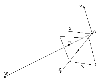
Figure 1: The pinhole camera model, with the camera reference frame ( X,Y,Z) depicted. Z is also called the optical axis.

A pinhole camera is modeled by its optical center C and its retinal plane (or image plane) $\cal R$. A 3-D point W is projected into an image point m given by the intersection of $\cal R$ with the line containing C and W.

Let ${\bf w} = (x,y,z)$ be the coordinates of W in the world reference frame (fixed arbitrarily) and ${\bf m}$ the pixel coordinates of m. In homogeneous (or projective) coordinates

$$\tilde{\bf m} = \left [ \begin{array}{c} u \\ v \\ 1 \\ \end{... ...[ \begin{array}{c} x\\ y\\ z\\ 1\\ \end{array}\right ]$$ (1)

the transformation from $\tilde{\bf w}$ to $\tilde{\bf m}$ is given by the matrix $\tilde{\bf P}$:

$$\kappa \tilde{\bf m} = \tilde{\bf P} \tilde{\bf w},$$ (2)

where $\kappa$ is a scale factor called projective depth. If $\tilde{\bf P}$ is suitably normalized, $\kappa$ becomes the true orthogonal distance of the point from the focal plane of the camera.

The camera is therefore modeled by its perspective projection matrix (henceforth simply camera matrix) $\tilde{\bf P}$, which can be decomposed, using the QR factorization, into the product

$$\tilde{\bf P}= {\bf A} [{\bf R}\;\vert\;{\bf t}] .$$ (3)

The matrix ${\bf A}$ depends on the intrinsic parameters only, and has the following form:

$${\bf A} = \left [ \begin{array}{c c c } \alpha_u & \gamma & u... ... 0 & \alpha_v & v_0 \\ 0 & 0 & 1 \\ \end{array}\right ] ,$$ (4)

where $\alpha_u = -fk_u$, $\alpha_v = -fk_v$ are the focal lengths in horizontal and vertical pixels, respectively (f is the focal length in millimeters, k_u and k_v are the effective number of pixels per millimeter along the u and v axes), (u₀, v₀) are the coordinates of the principal point, given by the intersection of the optical axis with the retinal plane (Fig. 1), and $\gamma$ is the skew factor.

The camera position and orientation (extrinsic parameters), are encoded by the $3\times3$ rotation matrix ${\bf R}$ and the translation ${\bf t}$, representing the rigid transformation that aligns the camera reference frame (Fig. 1) and the world reference frame.

   
Epipolar geometry

Let us consider the case of two cameras (see Fig. 2).

  

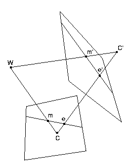
Figure: Epipolar geometry. The epipole of the first camera e is the projection of the optical center ${\sf C'}$ of the second camera (and vice versa).

If we take the first camera reference frame as the world reference frame, we can write the two following general camera matrices:

$$\tilde{\bf P} = {\bf A}[{\bf I}\vert {\bf0}] = [{\bf A} \vert {\bf0}]$$ (5)

$$\tilde{\bf P}^{\prime} = {\bf A}^{\prime} [{\bf R}\vert {\bf t}] .$$ (6)

A three-dimensional point ${\bf w}$ is projected onto both image planes, to points $\tilde{\bf m} = \tilde{\bf P} \tilde{\bf w}$ and $\tilde {\bf m}' = \tilde{\bf P}'\tilde{\bf w}$, which constitute a conjugate pair. From the left camera we obtain:

$$\begin{split} \kappa '\tilde{\bf m}^{\prime} &= {\bf A}^{\pri... ...\ z\\ \end{bmatrix} + {\bf A}^{\prime} {\bf t} . \end{split}$$ (7)

From the right camera we obtain: $\kappa {\bf A}^{-1} \tilde{\bf m}= [{\bf I}\vert {\bf0}] \; \tilde{\bf w} = [ x\; y\; z] ^\top.$Substituting the latter in (7) yields:

$$\begin{split} \kappa'\tilde{\bf m}^{\prime} &= \kappa{\bf A}^... ...}_\infty \tilde{\bf m} + \tilde{\bf e}^{\prime} \\ \end{split}$$ (8)

where ${\bf H}_{\infty} = {\bf A}'{\bf R}{\bf A}^{-1}$ and $\tilde {\bf e}' = {\bf A}'{\bf t}$ (the reason for this notation will be manifest in the following).

Equation (8) means that $\tilde{\bf m}^{\prime}$ lies on the line going trough $\tilde{\bf e}'$ and the point ${\bf H}_\infty \tilde{\bf m}$. In projective coordinates the collinearity of these three points can be expressed with the external product: $\tilde{\bf m}^{\prime \top} ( \tilde{\bf e}^{\prime} \wedge{\bf H}_\infty \tilde{\bf m}) =0 ,$ or

$$\tilde{\bf m}^{\prime \top} {\bf F} \tilde{\bf m} =0 ,$$ (9)

where ${\bf F} = [\tilde{\bf e}^{\prime}]_{\wedge}{\bf H}_\infty$ is the fundamental matrix, relating conjugate points, and $[\tilde {\bf e}^{\prime}]_{\wedge}$ is a matrix such that $\tilde{\bf e}^{\prime} \wedge{\bf x} = [ \tilde{\bf e}^{\prime} ]_{\wedge} {\bf x}.$ From (9) we can see that $\tilde{\bf m}^{\prime}$ belongs to the line ${\bf F} \tilde{\bf m}$ in the second image, which is called the epipolar line of $\tilde{\bf m}$. It's easy to see that $\tilde{\bf e}^{\prime \top}{\bf F} = {\bf0}$, meaning that all the epipolar lines contain the point $\tilde{\bf e}^{\prime}$, which is called the epipole (Fig. 2).

Since ${\bf F}\tilde{\bf e} = {\bf F}^\top\tilde{\bf e}' = {\bf0}$ the rank of ${\bf F}$ is in general two and, being defined up to a scale factor, it depends upon seven parameters. In the most general case, the only geometrical information that can be computed from pairs of images is the fundamental matrix. Its computation requires a minimum of eight point correspondences to obtain a unique solution [29,51].

It can be seen that (9) is equivalent to

$$({\bf A}^{\prime -1}\tilde{\bf m}^{\prime})^\top[{\bf t} ]_{\wedge}{\bf R} ({\bf A}^{-1} \tilde{\bf m}) = 0 .$$ (10)

Changing to normalized coordinates, $\tilde{\bf n} = {\bf A}^{-1}\tilde{\bf m},$ one obtain the original formulation of the Longuet-Higgins [27] equation,

$$\tilde{\bf n}^{\prime \top} {\bf E} \tilde{\bf n} = 0$$ (11)

involving the essential matrix

$${\bf E} = [{\bf t}]_{\wedge}{\bf R},$$ (12)

which can be obtained when intrinsic parameters are known. ${\bf E}$depends upon five independent parameters (rotation and translation up to a scale factor). From (10) it is easy to see that

$${\bf F} = {\bf A}^{ \prime -\top} {\bf E} {\bf A}^{-1} .$$ (13)

Unlike the fundamental matrix, whose only property is being of rank two, the essential matrix is characterized by the two constraints found by Huang and Faugeras [25] which are the nullity of the determinant and the equality of the two non-zero singular values. Indeed, the following Theorem holds:

Theorem 2.1   A real matrix ${\bf E}$ $3\times3$ can be factorized as product of a nonzero skew-symmetric matrix and a rotation matrix if and only if ${\bf E}$ has two identical singular values and a zero singular value.

For a proof see [13,8].

Homography of a plane

Given two views of a scene, there is a linear projective transformation (an homography) relating the projection ${\bf m}$ of the point of a plane ${\Pi}$ in the first view to its projection in the second view, ${\bf m}'$. This application is given by a $3\times3$ invertible matrix ${\bf H}_{\Pi}$ such that:

$$\tilde{\bf m}' = {\bf H}_{\Pi} \tilde{\bf m}.$$ (14)

It can be seen that, given the two projection matrices,

$$\tilde{\bf P}= {\bf A} [{\bf I}\;\vert\;{\bf0}], \;\;\; \;\;\;\tilde{\bf P}'= {\bf A}' [{\bf R}\;\vert\;{\bf t}]$$ (15)

(the world reference frame is fixed on the first camera) and a plane ${\Pi}$ of equation ${\bf n}^\top{\bf x} = d$, the following holds [30]:

$${\bf H}_{\Pi} = {\bf A}'({\bf R} + {\bf t} \frac{{\bf n}^\top}{d}){\bf A}^{-1} .$$ (16)

${\bf H}_{\Pi}$ is the homography matrix for the plane ${\Pi}$. If $d \rightarrow \infty$,

$${\bf H}_{\infty} = {\bf A}'{\bf R}{\bf A}^{-1} .$$ (17)

This is the homography matrix for the infinity plane, which maps vanishing points to vanishing points and depends only on the rotational component of the rigid displacement. It can be easily seen that:

$${\bf H}_{\Pi} = {\bf H}_{\infty} + \tilde{\bf e}' \frac{{\bf n}^\top}{d}{\bf A}^{-1}$$ (18)

where $\tilde{\bf e}' = {\bf A}'{\bf t} .$