 , in which drainage lines want to be characterized, comes back to 1852 and is owed to De Saint-Venant who identifies les faîtes et les thalwegs (watersheds/watercourses) as points of minimum slope (gradient magnitude
The older paper I have read , in which drainage lines want to be characterized, comes back to 1852 and is owed to De Saint-Venant who identifies les faîtes et les thalwegs (watersheds/watercourses) as points of minimum slope (gradient magnitude
 ![]() ) along a level curve of the relief [76]. De Saint-Venant's definition can be tested locally and it can be written [86, 12] in compact tensorial form as
) along a level curve of the relief [76]. De Saint-Venant's definition can be tested locally and it can be written [86, 12] in compact tensorial form as
De Saint-Venant's condition was also reformulated by Haralick [34]: height extrema in the direction having greatest second directional derivative magnitude. Being ![]() and
and ![]() the unit eigenvectors of the Hessian matrix of L, with
the unit eigenvectors of the Hessian matrix of L, with ![]() as corresponding eigenvalues, we know from standard calculus that
as corresponding eigenvalues, we know from standard calculus that
![]() are the directions in which the second directional derivative is extremized, and
are the directions in which the second directional derivative is extremized, and ![]() are the values of the extrema. Then, supposing we are not at any critical point of L, this is, under the requirement
are the values of the extrema. Then, supposing we are not at any critical point of L, this is, under the requirement
![]() , the new formulation can be formalized as [35]
, the new formulation can be formalized as [35]
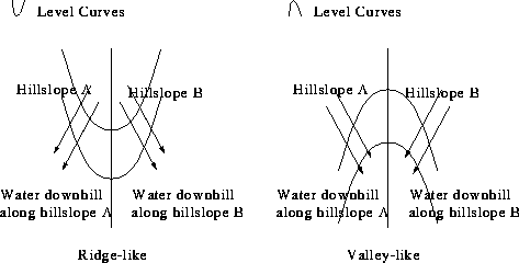
As is noticed in [45] this formulation is equivalent to De Saint-Venant's condition. On the other hand, De Saint-Venant's condition fails to detect the special slopelines that form the landscape's drainage pattern: the curvature of the slopelines
can be defined as ![]() , therefore,
, therefore, ![]() along a slopeline would imply that it is a straight line, which means that the special slopelines, where water accumulates, should be planar curves confined in vertical planes, clearly in conflict with our experience. This was noticed by Boussinesq [8] and Breton
de Champ
along a slopeline would imply that it is a straight line, which means that the special slopelines, where water accumulates, should be planar curves confined in vertical planes, clearly in conflict with our experience. This was noticed by Boussinesq [8] and Breton
de Champ  [9].
[9].

Figure 2: The loci of level curve curvature extrema have been proposed as candidates
to form the drainage pattern and the inverse drainage pattern.
Other typical local crease detector, that has been claimed to characterize the loci where water gathers to run downhill (or the dual loci by turning the relief upside down) [47], looks for maxima of the absolute value of the curvature of the relief's level curves. Notice in figure 2 how, visually, it is a reasonable assumption that these points are the loci where water converge/diverge. The curvature of the level curves can be defined in terms of the landscape derivatives as ![]() . It is a signed quantity whose sign classifies the surface as convex (
. It is a signed quantity whose sign classifies the surface as convex ( ![]() ) or concave (
) or concave ( ![]() ) with respect to the vertical direction (height). In [25, 91, 90, 17] it is formulated the extremality condition
) with respect to the vertical direction (height). In [25, 91, 90, 17] it is formulated the extremality condition

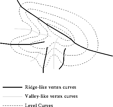
Figure 3: Vertex curves: extrema of ![]() along the level curve tangent direction, level by level.
along the level curve tangent direction, level by level.

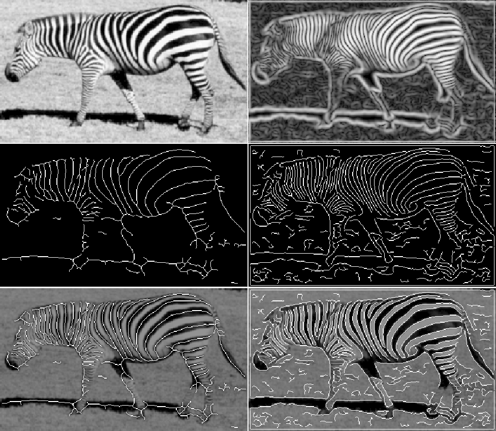
Figure 4: From top to bottom and left to right: (a) Zebra on a grass background. Black fringes are valleys, white fringes are ridges. (b) Edgeness image from the zebra, consisting of its gradient magnitude. The centers of the ridges of this image are edges of the zebra: boundary between black and white streams. The edgeness at the silhouette of the zebra is not as high as we would like, since for that we should use a texture gradient measure. (c) Valley-like structures from the zebra, which have been extracted just by thresholding ![]() according with the implementation given in [52], and discarding short segments. (d) Ridge-like structures from the edgeness image computed in the same way than the previous valley-like structures. (e) Valley-like structures over the zebra. The dynamic range of the zebra's grey-values have been reduced for visualization purposes. (f) Edges from the ridge-like structures of the edgeness image, superposed on the zebra.
according with the implementation given in [52], and discarding short segments. (d) Ridge-like structures from the edgeness image computed in the same way than the previous valley-like structures. (e) Valley-like structures over the zebra. The dynamic range of the zebra's grey-values have been reduced for visualization purposes. (f) Edges from the ridge-like structures of the edgeness image, superposed on the zebra.
These extrema are connected from one level to the next and form the so-called vertex curves or extremal curvature curves (ridge and valley like curves together, figure 3). A remarkable fact is that extrema of ![]() are directly connected with the medial axis concept through Leyton's duality theorem [50]: given a planar curve (e.g. a level curve) and a curvature extremum along it, no matter which of the differential symmetry analyzes one chooses, there has to be a unique symmetry axis terminating at the extremum. As we mentioned in section 3, by stacking the medial axis of each level curve we obtain a skeleton of the landscape called IAS. Then, the set of top/bottom curves of the IAS have a one-to-one relationship with vertex curves.
are directly connected with the medial axis concept through Leyton's duality theorem [50]: given a planar curve (e.g. a level curve) and a curvature extremum along it, no matter which of the differential symmetry analyzes one chooses, there has to be a unique symmetry axis terminating at the extremum. As we mentioned in section 3, by stacking the medial axis of each level curve we obtain a skeleton of the landscape called IAS. Then, the set of top/bottom curves of the IAS have a one-to-one relationship with vertex curves.
From a hydrologic point of view, the ![]() based definition also fails to detect the special slopelines that form the landscape's drainage pattern [45]. Furthermore,
based definition also fails to detect the special slopelines that form the landscape's drainage pattern [45]. Furthermore, ![]() based creases, opposite to De Saint-Venant based, are invariant under the general group of monotonic height (grey-level) transforms [22, 17]. Besides, both the De Saint-Venant's definition and the
based creases, opposite to De Saint-Venant based, are invariant under the general group of monotonic height (grey-level) transforms [22, 17]. Besides, both the De Saint-Venant's definition and the ![]() based method give creases that are invariant under rotations and translations of the spatial axes, as well as uniform scaling [17].
based method give creases that are invariant under rotations and translations of the spatial axes, as well as uniform scaling [17].

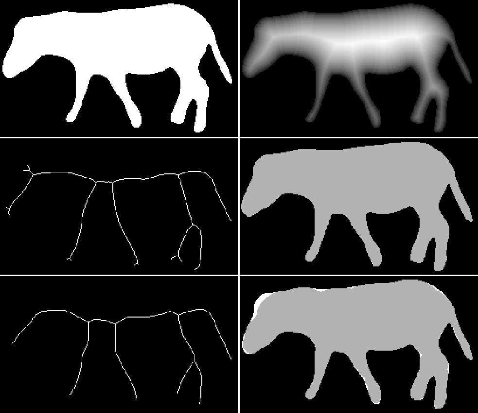
Figure 5: From top to bottom and left to right: (a) Binary image: white object. (b) Medialness measure, according with a Gaussian smoothing of the Chamfer distance from the interior points to the border of the object. The SA appears as a ridge-like structure. (c) SA: Ridge-like structures from
the Medialness measure, which have been extracted by just thresholding ![]() according with the implementation given in [52], and discarding short segments. On the other hand, there exist specific algorithms for ridge-like extraction from medialness measures
of binary objects [2]. (d) Reconstructed object from the SA and the Medialness image: at each pixel of the image, if it belongs to the SA we draw a circle whose radius is given by the grey-value of the corresponding pixel at the Medialness measure. Grey: reconstructed object. White: difference with the original. (e) SA: computed by means of a thinning algorithm [96]. (f) Reconstructed image from (e). Comparing the result
with (d) we see that the SA based on the extraction of ridge-like structures of a medialness measure encodes better the shape than the one based on a thinning algorithm.
according with the implementation given in [52], and discarding short segments. On the other hand, there exist specific algorithms for ridge-like extraction from medialness measures
of binary objects [2]. (d) Reconstructed object from the SA and the Medialness image: at each pixel of the image, if it belongs to the SA we draw a circle whose radius is given by the grey-value of the corresponding pixel at the Medialness measure. Grey: reconstructed object. White: difference with the original. (e) SA: computed by means of a thinning algorithm [96]. (f) Reconstructed image from (e). Comparing the result
with (d) we see that the SA based on the extraction of ridge-like structures of a medialness measure encodes better the shape than the one based on a thinning algorithm.
Whatever crease detector we use, since creaseness is a local feature, we need a grouping process if we want to have creases as curves (similarly for higher dimensions). We can perform the detection of crease points and their grouping at the same time: from a given crease point we look for other at its neighborhood according with some set of grouping rules or following some numerical scheme [38, 88, 54, 53, 4]. Other possibility consist of a first step extracting crease points and a post-processing step grouping them [33, 83].
Both the De Saint-Venant and the level curve curvature based definitions fail to characterize the special slopelines that form the drainage pattern of a landscape. However, the different characterizations of creases have been proved to be a very important image feature in applications as fingerprint analysis [14, 56, 39], road detection in aerial and infra-red images [33, 79, 61, 83, 49], extraction of features for character and/or digit recognition from grey-level images [95, 48, 92], surface interrogation [37, 38], feature detection in range images [27, 70, 69], analysis of the landscape abruptness [47, 77], registration of brain images based on anatomical landmarks [19, 20, 55, 88, 91, 31, 32], medical image analysis [26, 25, 63, 3, 4], etc. Moreover, the definition of 1D creases (curves) in a 2-dimensional landscape has been extended to compute k- creases in d-dimensional spaces (k < d and ![]() ) by Eberly [18, 17]. For example, in the computation of MMA it is used the 'height definition' of creases, which is the extension of De Saint-Venant's idea to d-dimensional images, by generalizing (2).
In figure 4 we can see an example of crease extraction from both an image with a zebra and the gradient magnitude of the image (edgeness). In figure
5 we see an example of crease extraction from a medialness measure.
) by Eberly [18, 17]. For example, in the computation of MMA it is used the 'height definition' of creases, which is the extension of De Saint-Venant's idea to d-dimensional images, by generalizing (2).
In figure 4 we can see an example of crease extraction from both an image with a zebra and the gradient magnitude of the image (edgeness). In figure
5 we see an example of crease extraction from a medialness measure.