 Mean and Gaussian
Curvature

So far, we have shown that a surface may be characterised by 6 functions, E, F, G, L, M and N. We have also shown that the information
from these 6 functions can be ``reduced'' into two curvature functions  and
and  . Information has been lost, but curvature is a useful method of describing and classifying surfaces,
or alternatively collections of points within a depth image which may be grouped together to form a surface which may be part of an object model.
Whereas the principal curvatures are associated with the principal directions at a point on a surface, it is possible to combine these into direction independent quantities, the Gaussian, K, and mean, H, curvatures.


 and
and  are roots of the quadratic equation,

or

The mean and Gaussian curvatures are important quantities in computer vision because they provide a common method of specifying eight basic
types of surface with these visible invariant properties. These are tabulated below, and illustrated in Figure 3.
The method based on  and
and  is less common as they are dependent on direction. Of course, the problem with surface classification in the real world is knowing where to set the thresholds.
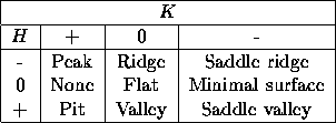
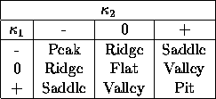
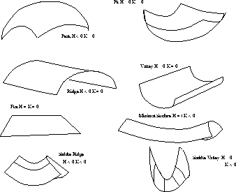
Figure 3: Surface classification using HK signs
Re-arrangement and combination of the several equations above yields several different expressions to compute H and K.
In summary, the five partial derivatives,  ,
,  ,
,  ,
,  ,
,  are all we need to compute the six fundamental form coefficients E,F,G,L,M,N and
hence the mean and Gaussian curvature


There are several other features which are useful for surface characterisation and range image segmentation. For example, the metric determinant is the square root of the determinant of the first fundamental form matrix,

This could be considered as a measure of edge magnitude as it is approximately the square root of the sum of the squares of the
partial derivatives, and is thus similar to a gradient edge detector. A threshold on depth provides a detector for blade (but not fold) edges.
The summation is the surface area

Similarly, the quadratic variation gives a second useful measure.

When summed over an area, this gives a measure of the flatness of a region; however it does depend on viewpoint.
Techniques for segmentation of 3D data may be similar in principle to techniques for 2D regional segmentation; they may be based on local
growing from a seed (e.g. blob colouring), or more global transformation (Hough). In general, we can use the explicit form for segmenting images, and in particular graph surfaces since depth data is often acquired from a single viewpoint. If we build 3D descriptions from
several viewpoints, for example by rotating an object on a turntable to obtain an ``all-round'' depth map, then we may be better advised to use
the implicit form.
For example, consider the problem of finding planes in a depth image. Within a single image, planes can be specified by three parameters,
A,B and C in Equation 2. One approach to planar segmentation, based on the three point seed algorithm starts from a set of three points, fitting the exact plane which passes through them. Provided these three points
are not collinear then there should only be one solution. Then the approach attempts to add adjacent points to the plane either measuring a metric distance between these points and the fitted plane, or possibly recomputing a least squares fit on more than 3 points and computing the residual error. Provided the planar fit remains good, and all points can be included in the plane then the planar region grows in a manner similar to the blob colouring approach we discussed earlier.
Alternatively, we could use a Hough transform on all data points concurrently. Using single depth points we could compute the A,B and C parameters of the set of possible planes passing through each point, and enter them in the accumulator array; planes are detected by peaks in parameter space as before. To constrain the mapping from image to parameter space to a one-to-one form, we
could take sets of three points and compute the normal, or fitted plane, as before.
In general, a depth image will not only contain planes, so we have to fit higher order surfaces as well. Often the question arises; should we attempt to find typed second order surfaces, such as cylinders and cones, or use the more general quadric form ? Furthermore, how should we progress to find surfaces ? For example, it is common to attempt to fit all planar surfaces first, then progress
to more complex forms for unclassified surfaces. This may well affect the final segmentation, since it may be possible to fit either a plane, say, or a cylinder of small curvature to the same set of data points.
Of course, we can use the classification based on HK parameters to provide a segmentation of an image. As an example,
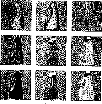
Figure 4, below, shows progressive processing of an image of a bottle of washing up liquid, taken from an article by Li
in the International Journal of Computer Vision. This shows the partial derivatives and a histogram of the K (above) and H (below)
parameters in the top line. The middle line shows an initial classification based on thresholds derived from the histograms. From left to right we have H values (- is dark, 0 is middle, + is light ), K values and the HK classifcation. The bottom line shows the final values after an iterative process based on smoothness constraints. In the final figure, for example, the bulk of the bottle is a ridge, the dark area near the top is
a peak, and the light patch round the handle is a saddle ridge.

Figure 4: Segmentation based on HK parameters
Although it is conceivable that models may be built from HK patches, this is rarely the case in practice. We now consider
fitting surfaces to an already existing segmentation, e.g. the classified sets of points using HK parameters. Thus we assume that the problem is simply to fit the required surface, in either planar or quadric form. This is not necessarily the best approach, and in practice it is probable that the point groupings will change as the fit is shown to be not good. However, it illustrates one possible method.
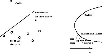
We consider a least squares approach: i.e. we wish to minimise the sum of the squared errors between the fitted surface and the data points. The least squares approach has one noted weakness; it does not handle outliers well. It assumes that the errors follow a Gaussian distribution; if a single point lies well outside this error range it can severely distort the eventual
fit (Figure 5, below).
There are several ways to counteract this problem, e.g. random sampling of point subsets, robust statistics or pre-processing the depth data by a robust operator, for example a median filter. We shall assume here that outliers have been removed by the latter process.
The next problem we would wish to consider is the error metric. How do we compute the error between a depth point and the fitted surface? Figure 5 illustrates this point; there are at least two plausible choices of error measure in a depth image, the z distance since this is what we measure and may be assumed to have a Gaussian distribution, or the distance to the fitted surface which is viewpoint independent. The former is the algebraic distance and is the one we shall use as it is computationally simpler. The latter is the geometric distance; this is arguably a better metric, but is computationally more difficult when considering higher order surfaces.

Figure 5: The Least Squares approach: some problems


[ Surface description and differential geometry |
The exact fit ]
Comments to: Sarah Price at ICBL.
 and
and  . Information has been lost, but curvature is a useful method of describing and classifying surfaces,
or alternatively collections of points within a depth image which may be grouped together to form a surface which may be part of an object model.
Whereas the principal curvatures are associated with the principal directions at a point on a surface, it is possible to combine these into direction independent quantities, the Gaussian, K, and mean, H, curvatures.


 and
and  are roots of the quadratic equation,


 and
and  is less common as they are dependent on direction. Of course, the problem with surface classification in the real world is knowing where to set the thresholds.


 ,
,  ,
,  ,
,  ,
,  are all we need to compute the six fundamental form coefficients E,F,G,L,M,N and
hence the mean and Gaussian curvature


