

The attributed relational graph
Robustness of the representation
A good object representation is a description of object/objects by high level features from all perspectives, both spatial and temporal. Extensive representations have been proposed to model objects. They can roughly be categorized as global representation and local representation. Examples of global representations include: color appearance model, subspace methods (like PCA [1]), etc. Local representation describes the object using a set of local features, which are usually selected as the local characterization of object parts. This kind of representation usually incorporates relations between local features to capture the object structure. Typical such representation is region adjacent graph [2]. However, relative less work has been done on modeling the dynamic changes of the object model. Dynamic feature graph is designed as a representation that models both spatial and temporal characteristics of an object. Spatially, the object is represented as an attributed relational graph [3], with features as nodes and their relations as the edges. Temporally, the graph can adaptively update itself to keep the good features and eliminate unstable features.
Graph representations are widely used for dealing with structural information in different domains such as psycho-sociology, image interpretation and pattern recognition. Attributed relational graph is a more powerful approach for image representation than pure feature based representations. The semantic information of the relationships among the image features is represented by the attributes associated with the relations between their corresponding features. This approach for image representation has shown to provide compact, concise and powerful representation that is capable of comprehending rich information contents of the images. The attributed relational graph is defined as follows:
![]() is
a relational graph.
is
a relational graph.
![]() is
the node set.
is
the node set.
![]() is
the edge set.
is
the edge set.
where the nodes can be point features, region features, etc. Each node is associated with a set of properties like position, color, etc, called the attributes to describe the feature characteristics. Correlated features are usually connected with edges. The edges represents the geometric relationship of the features, which can be the distance or scale between adjacent features. Usually, features that are close enough to each other are called correlated and edges between them are formed . Example of an attributed relational graph with the SIFT (Scale Invariant Feature Transform) as the feature is shown in Figure 1.
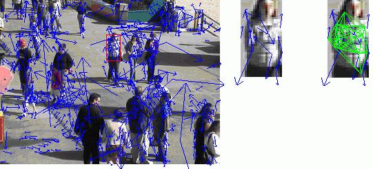
Figure 1. Attributed relational graph.
The left image is the scene with the SIFT features imposed by blue arrows (denote attributes of features with different position, scale and orientation); the middle figure is the scaled version of the red rectangle area; the right image is the relational graph, with the green lines showing the edges.
Over time, the object modeled by the relational feature graph may change it's appearance significantly dramatically due to the illumination condition changes, pose changes, etc. Features that are characteristic in some frames maybe be completely out of view in the next frames. The dynamic feature graph models this kind of temporal changes by swapping in and out features to keep the best features in the model. The goodness of a feature is measured as the stability over time. This adaptively evolving scheme keep the optimal object representation even when the object has undergone significant changes. Since both the graph nodes and edges evolve over time, their dynamics should be modeled simultaneously. However, the edges are fully dependent on nodes, and once nodes are determined, edges can be uniquely determined. So, we only need to model the node dynamics to incorporate the relation dynamics.
Since in each frame, new features may show up due to the
appearance changes or pose changes, it’s not wise to treat newcomers equally
with the features that have been proved to be stable. We need a scheme to
temporarily hold the new features, and after some period of competition, boost
those really stable features into model. So, we also maintain a candidate
feature set to hold potential stable features. Each feature has an
associated status vector, identifying on which frame it appears and on which
frame not. We assume the probability for the features in the candidate set to be
added into the model with a Binomial distribution
![]() where is the time window we use for
evaluating the feature stableness.
where is the time window we use for
evaluating the feature stableness.
![]() is the
probability that the feature is observed. For efficiency concerns, in each
frame, only those features whose probability of being boosted are higher than a
threshold
is the
probability that the feature is observed. For efficiency concerns, in each
frame, only those features whose probability of being boosted are higher than a
threshold
![]() can be added into the model. That
is
can be added into the model. That
is
![]() truncated betweenwhere is the number of times the
feature is observed in the previous frames.
This candidate feature set must be updated in each frame after the state has
been updated.
truncated betweenwhere is the number of times the
feature is observed in the previous frames.
This candidate feature set must be updated in each frame after the state has
been updated.
Due to object pose or illumination changes, the features which have been stable for previous frames may become inactive in the future. A scheme for deleting such in-active features is incorporated into our framework. For those features already in the model, we also maintain a history of their performances on the previous frames, if a feature has not been matched for quite some times, we consider it to be inactive and delete it from the model (stable feature set). Similar to the scenario to incorporate new features, we also model the feature deletion as a Binomial distribution: truncated between whereis the number of times the feature is missed in the frames, is the minimum probability that the feature can be deleted from the model.
The model feature addition and deletion is a survival of the fittest scheme. Figure 2 is a simplified demonstration of this model update process. It always keeps good features (in terms of stableness) in the model. This competitive strategy greatly enhances the flexibility of the model, which makes it more suitable for tracking under appearance and pose changes.
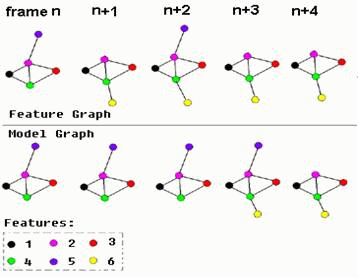
Figure 2, Dynamic model update
Graph nodes are shown as colored circles, and the edges are the lines connecting them. The first row is the observation from image sequence; the second row is the object model at each frame. At frame n, the model contains 5 feature(1-5). In the 5 frames n to n+4, the blue feature(5) is observed only twice, so it is selected as an unstable feature and deleted from the model (second row) at frame n+4. And at frame n+3, the new feature 6 has been persistently observed for 3 consecutive frames, so, it is a stable feature, and is selected from candidate set. (For simplicity, the candidate set is not drawn in the figure)
For a good object representation, we want it to be robust to various changes like the illumination changes, pose changes, partial occlusion, etc. The robustness of a dynamic feature graph comes from two aspects. One is the invariance property of the attributes of the features, the other is the robust and consistent of the feature detector. Under different conditions, the same feature may have different appearance, good attributes are invariant to these changes. This means the stableness of the nodes in the graph representation. The consistent of the feature detector means the robustness of the graph edges. Because edges are usually determined by the relative positions of features, robust feature detector can keep detection the feature consistently over time.
The dynamic feature graph has been applied to model dynamically changing objects in tracking [4]. The object is described using a collection of SIFT features; the relations between features are encoded as the edges in the attributed graph. The graph dynamics is modeled with the feature/relation addition and deletion using a high order HMM which provides a competitive mechanism that can always keep the stable features in the model. The likelihood computation is formulated into a graph matching problem that can be efficiently solved using relaxation labeling [5]. Figure 3 demonstrates the tracking results of a pedestrian under appearance changes and occlusion.
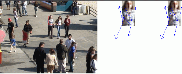
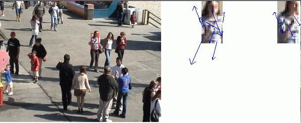
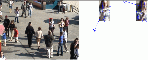
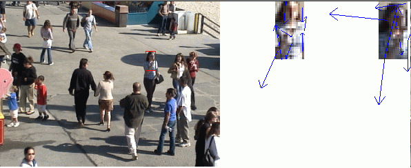
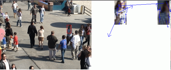
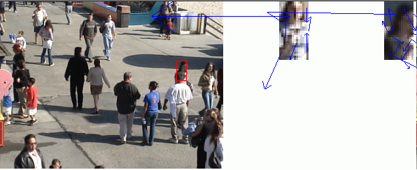
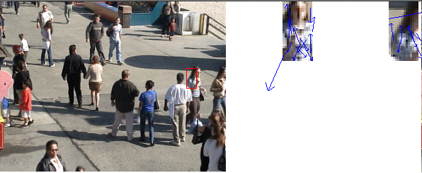

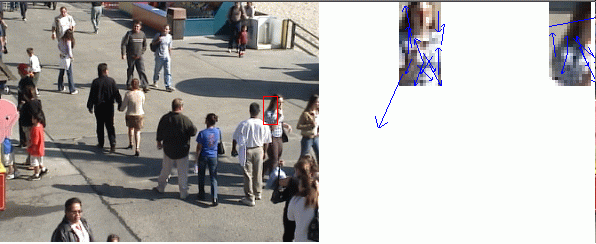

Figure 3 Tracking of a pedestrian under significant appearance changes and heavy occlusion
The red rectangles are the tracked position, and the model and clipped tracking results with SIFT features (blue line with arrow) overlaid are shown on the side next to the scene image. the right most small image is the visualization of the current dynamic feature model.
More tracking results:
Pedestrian tracking with appearance changes and heavy occlusion
Vehicle tracking under heavy occlusion
Vehicle tracking with pose changes and appearance changes
[1] http://homepages.inf.ed.ac.uk/rbf/CVonline/LOCAL_COPIES/FISHER/PCA/pca.html
[2] http://homepages.inf.ed.ac.uk/rbf/BOOKS/FSTO/node10.html
[3] M A Eshera, K S Fu "An image understanding system using attributed symbolic representation and inexact graph-matching" IEEE PAMI Volume8, Issue 5 Pages: 604 - 618 (September 1986)
[4] Feng Tang, Hai Tao "Object tracking with dynamic feature graph" VS-PETS, in conjunction with ICCV, Beijing, October, 2005
[5] http://homepages.inf.ed.ac.uk/rbf/CVonline/LOCAL_COPIES/MARBLE/high/matching/relax.htm