Likelihood criterion

Drawing a tiny, random subset of all features, we can safely assume individual samples to be statistically independent of each other. The logarithmic likelihood of object $O$, described by database histogram $H_O$, given the sensed subsample ${\cal{S}}_{O'}$ of features, thus is

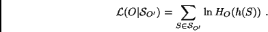$${\cal{L}}(O \vert {\cal{S}}_{O'}) = \sum_{S \in {\cal{S}}_{O'}} \ln H_{O}(h(S))\ .$$ (16)

The mapping $h(S)$ is as defined in Equation (9). In contrast to the Kullback-Leibler divergence (15), all logarithms can here be calculated in the training phase and logarithmic histograms $\ln H_{O}$ can be stored.

Figure 2: The 20 objects of the database.

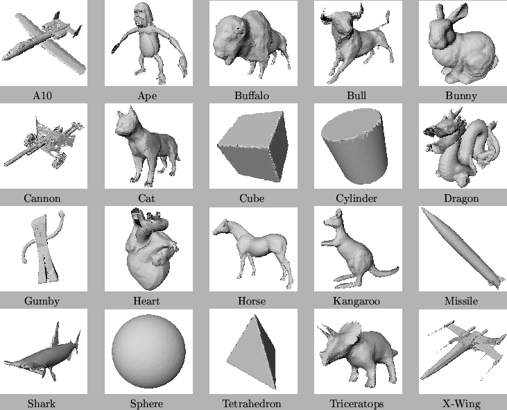Table 1: In this test, the six classifiers defined in Section 4 are evaluated using randomly drawn feature samples from complete and noise-free surface meshes of the 20 objects shown in Figure 2. Achieved recognition rates are given in percent. The processing times are measured on a standard PC with an Intel Pentium IV 2.66 GHz processor and Linux as operating system.

criterion	recognition in %	time in ms
$\bigcap$	42.7	5.12
${\cal{E}}$	40.6	5.01
$\chi_1^2$	75.4	6.16
$\chi_2^2$	45.5	6.25
${\cal {K}}$	99.6	7.42
${\cal {L}}$	99.7	4.79

Figure 3: The six arrays represent classification results for the 20 objects shown in Figure 2 using the six different criteria defined in Section 4. Surfaces are completely visible and data are noise free. In each array, columns represent test objects, rows trained objects. Grey values indicate the rate of classification of a test object as a trained object; a brighter shade means a higher rate. The more distinct the diagonal, the higher the allover performance of the classifier. Evidently, the ${\cal {K}}$ and ${\cal {L}}$ criteria achieve almost perfect classification within our database of objects.

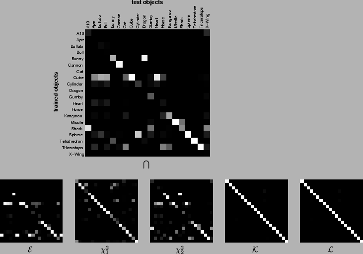Figure 4: (a) X-wing; (b) X-wing with noise (4%); (c) partially visible X-wing (33%).

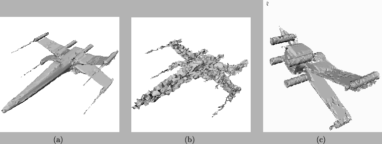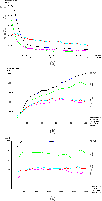
Figure 5: Plots of recognition rates for the 20 objects shown in Figure 2 using the six different criteria defined in Section 4. The conditions for the test data are varied; (a) varying level of noise (in percent of maximal object diameter); (b) varying visibility (in percent of complete surface area); (c) varying mesh resolution (in percent of training resolution). The curves for the ${\cal {K}}$ and ${\cal {L}}$ criteria nearly coincide in all three graphs.