The Process Model
In this simple example let us attempt to estimate a scalar random constant, a voltage for example. Let's assume that we have the ability to take measurements of the constant, but that the measurements are corrupted by a 0.1 volt RMS white measurement noise (e.g. our analog to digital converter is not very accurate). In this example, our process is governed by the linear difference equation
 ,
,
with a measurement  that is
The Simulations
To begin with, we randomly chose a scalar constant  (there is no "hat" on the z because it represents the "truth"). We then simulated 50 distinct measurements
  that had error normally distributed around zero with a standard deviation of 0.1 (remember we presumed that the measurements are corrupted by a 0.1 volt RMS white measurement noise). We could have generated the individual measurements within the filter loop, but pre-generating the set of 50 measurements allowed me to run several simulations with the same exact measurements (i.e. same measurement noise) so that comparisons between simulations with different parameters would be more meaningful.
In the first simulation we fixed the measurement variance at  . Because this is the "true" measurement error variance, we would expect the "best" performance in terms of balancing responsiveness and estimate variance. This will become more evident in the second and third simulation.
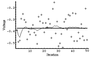
Figure 3-1
depicts the results of this first simulation. The true value of the random constant
  is given by the solid line, the noisy measurements by the cross marks, and the filter estimate by the remaining curve.
Figure 3-1.
The first simulation:
 . The true value of the random constant
  is given by the solid line, the noisy measurements by the cross marks, and the filter estimate by the remaining curve.
When considering the choice for  above, we mentioned that the choice was not critical as long as
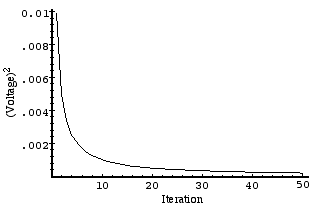
  because the filter would eventually converge. Below in
Figure 3-2
we have plotted the value of
  versus the iteration. By the 50th iteration, it has settled from the initial (rough) choice of 1 to approximately 0.0002 (Volts2).
Figure 3-2.
After 50 iterations, our initial (rough) error covariance
 choice of 1 has settled to about 0.0002 (Volts2).
In
section
under the topic
"Filter Parameters and Tuning"
we briefly discussed changing or "tuning" the parameters Q and R to obtain different filter performance. In
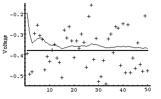
Figure 3-3
and
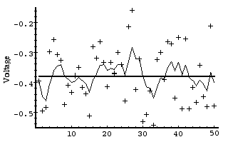
Figure 3-4
below we can see what happens when R is increased or decreased by a factor of 100 respectively. In
Figure 3-3
the filter was told that the measurement variance was 100 times greater (i.e.  ) so it was "slower" to believe the measurements.
Figure 3-3.
Second simulation:
 . The filter is slower to respond to the measurements, resulting in reduced estimate variance.
In
Figure 3-4
the filter was told that the measurement variance was 100 times smaller (i.e.  ) so it was very "quick" to believe the noisy measurements.
Figure 3-4.
Third simulation:
 . The filter responds to measurements quickly, increasing the estimate variance.
While the estimation of a constant is relatively straight-forward, it clearly demonstrates the workings of the Kalman filter. In
Figure 3-3
in particular the Kalman "filtering" is evident as the estimate appears considerably smoother than the noisy measurements.
 ,
, that is
 .
. . There is no control input so
  . Our noisy measurement is of the state directly so
  . (Notice that we dropped the subscript k in several places because the respective parameters remain constant in our simple model.)
 ,
, ,
, (3.1)
(3.1) ,
, .
. . (We could certainly let
  but assuming a small but non-zero value gives us more flexibility in "tuning" the filter as we will demonstrate below.) Let's assume that from experience we know that the true value of the random constant has a standard normal probability distribution, so we will "seed" our filter with the guess that the constant is 0. In other words, before starting we let
  .
. , i.e.
  . If we were absolutely certain that our initial state estimate
  was correct, we would let
  . However given the uncertainty in our initial estimate
  , choosing
  would cause the filter to initially and always believe
  . As it turns out, the alternative choice is not critical. We could choose almost any
  and the filter would eventually converge. We'll start our filter with
  .
.  (there is no "hat" on the z because it represents the "truth"). We then simulated 50 distinct measurements
  that had error normally distributed around zero with a standard deviation of 0.1 (remember we presumed that the measurements are corrupted by a 0.1 volt RMS white measurement noise). We could have generated the individual measurements within the filter loop, but pre-generating the set of 50 measurements allowed me to run several simulations with the same exact measurements (i.e. same measurement noise) so that comparisons between simulations with different parameters would be more meaningful.
 . Because this is the "true" measurement error variance, we would expect the "best" performance in terms of balancing responsiveness and estimate variance. This will become more evident in the second and third simulation.
  is given by the solid line, the noisy measurements by the cross marks, and the filter estimate by the remaining curve.
 . The true value of the random constant
  is given by the solid line, the noisy measurements by the cross marks, and the filter estimate by the remaining curve.
 above, we mentioned that the choice was not critical as long as
  because the filter would eventually converge. Below in
  versus the iteration. By the 50th iteration, it has settled from the initial (rough) choice of 1 to approximately 0.0002 (Volts2).
 choice of 1 has settled to about 0.0002 (Volts2).
 ) so it was "slower" to believe the measurements.
 . The filter is slower to respond to the measurements, resulting in reduced estimate variance.
 ) so it was very "quick" to believe the noisy measurements.
 . The filter responds to measurements quickly, increasing the estimate variance.