As an introduction to the research I have been doing using and developing belief network approaches, I thought it might be useful to provide a basic introduction to what I am talking about. If you find this tutorial useful then please put a link to it on your home page. To switch to a printable form of this document hit here. Reload to return to the original form.
Belief Networks and Probabilistic Graphical Models
Belief networks (Bayes Nets, Bayesian Networks) are a vital tool in probabilistic modelling and Bayesian methods. They are one class of probabilistic graphical model. In other words they are a marriage between two important fields: probability theory and graph theory. It is this combination which makes them a powerful methodology within machine learning and statistics.
Use of belief networks has become widespread partly because of their intuitive appeal. A given belief network is very easily related to a particular probabilistic model, and is easily understood in turns of direct dependence. Because they are useful in simplifying the manipulations in Bayesian inference they have a great practical use in real world problems. Belief networks, or Bayes Nets as they are sometimes known, have been used widely from medical diagnosis to image modelling, from genetics to speech recognition, from economics to space exploration. They can be valuable in any area where there is the requirement for finding out about unknown variables through the utilisation of structural relationships and data. Even if the exact form of the relationships between the variables of interest are not known it does not matter, because the uncertainty can be represented probabilistically.
Introduction to Bayesian Methods
Although belief networks are a tool of probability theory, their most common use is within the framework of Bayesian analysis. This is one reason they are often called Bayesian networks (more importantly Bayes theorem is at least implicitly used in calculations with Bayes nets). The Bayesian approach is based on three fundamental beliefs:
- In order to infer anything from data, we must have and use prior information.
- Most problems involve some levels of uncertainty.
- Probability theory is the best (or a good) way of representing uncertainty because of Bayes theorem.
One implication of these beliefs is that there is no indisputable way of obtaining knowledge from data. There is a significant philosophical gulf between this belief and the foundationalist beliefs of the empiricists which led to the development of frequentist statistics.
The Bayesian approach to problems can be summed up in this simple way:
- Suppose we have some sets of variables of interest, Q and D.
- We use prior knowledge to define a probability distribution P(Q,D) over the variables of interest.
- We then receive some data telling us what values D takes.
- We update our belief about Q by calculating P(Q|D), the probability of Q given we know what D is.
The big issues in Bayesian methods involve how to find out what form P(Q,D) should take, and how to calculate P(Q|D). Belief networks help with both of these problems.
Belief Networks
Belief Networks use a graphical representation to represent probabilistic structure. There is a direct relationship between a graphical model and a particular form of probability distribution.
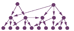 A belief network is a directed graph. That is, it consists of vertices (or nodes) and directed edges (arrows). Each edge points from one node (called the parent) to another node (known as the child). In a belief network each node is used to represent a random variable, and each directed edge represents an immediate dependence or direct influence. Although not strictly correct, one of the easiest ways to start thinking about belief networks is in term of causal (but not deterministic) dependence. For example we might be interested in diagnosing whether the household dog has fleas! There are some obvious variables which we would want to include in modelling this scenario: how much the dog is scratching (observable), whether the dog is molting (hidden), whether there are an excess of dog hairs around the house (observable),
  whether the cat has recently had fleas (observable) etc. We can build a belief network of this scenario by thinking in terms of causal relationships. We use these causal relationships to specify the direct dependencies in the graphical model.
For example, if the dog is molting then this would probably cause some increase in the amount of scratching, and also an increase in the number of dog hairs around the house. Fleas would also probably cause the dog to itch more. The fact that the cat has had fleas might cause our dog to get fleas too, if they had been in contact. We can use this information to specify the form of graphical model to the right. Note that this is not the 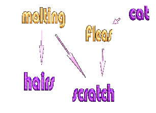 'right' graphical model; it is merely one way of describing the dependence relationships. Indeed we have neglected some direct dependence which might (or perhaps should) have been included; for example scratching will probably increase the number of hairs about irrespective of the cause of that scratching. Also, we will see later that the same probability distribution can be specified using many different graphical models. Even so, this causal approach is a useful way of thinking about graphical models in the beginning.
There can be a question as to how to choose what variables to include. Surely at the end of the day the whole world needs to be included in the belief network, at least in theory? In fact this is not the case. It is possible to marginalise, or integrate out, the effects of certain random variables. This means that the effect of the marginalised random variable is incorporated in the remaining variables and the conditional distributions which remain. On the other hand it is possible to assume other variables to be fixed - we might be only considering a limited scenario, for example we might assume we are on planet earth and therefore do not have to consider variations in the gravitational force! In theory then, given a finite belief network, one is assuming that the each part of the `rest of the universe' has been taken to be fixed or has been integrated out!
Although the belief network is related to the prior probability distribution we need to build, it does not fully specify it. What it does give is the conditional dependencies in the probability distribution. Given a belief network a minimum set of conditional independencies can be found using a rule called D-separation. On top of these direct dependence relationships, we need to give some numbers (or functions) which define how the variables relate to one another. In order to see how this works it is best to look first at the relationship between a belief network and a probability distribution.
A joint probability distribution P(A,B,C,D,E) over a number of variables can be written in the following form using the chain rule of probability:
P(A,B,C,D,E) = P(A) P(B|A) P(C|B,A) P(D|C,B,A) P(E|D,C,B,A). - (eq. 1)
Sometimes a probability distribution is not so general; that is there are a number of conditional dependencies which might arise. For example if we know A, C might no longer depend on what value B takes. Other such conditional dependencies could occur which enable use to write the probability in a simpler form - something like
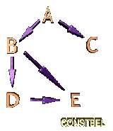
P(A,B,C,D,E) = P(A) P(B|A) P(C|A) P(D|B) P(E|D,B). - (eq 2)
The key is that this form of probability representation directly relates to a particular belief network. This belief network can be constructed in the following way.
- For each element of the above product we build a node of the network. For example for P(C|A) we create a node corresponding to the random variable A.
- For each element of the above product, we connect the relevant node to the nodes which that variable depends on. These nodes become the parents of the relevant node. For example, for the factor P(E|D,B) we would draw a directed edge from the node D to the node E and another directed edge from the node B to the node E.
Hence the whole belief network would look like figure CONSTBEL.
 This is how a belief network represents conditional independencies. If there are no conditional dependencies then the belief network is fully connected. A quick look at the form of equation 1 will also show that there are many different belief networks corresponding to one probability distribution. This is because we can permute A,B,C,D and E and reapply the chain rule. This will give a different root node and different structures. The key is to choose a representation which allows the conditional independence relationships to be utilised in the best way possible.
It is worth making a note about a causal view of belief networks at this point. There are a number of ways that this view is problematic. The first is that there are many ways of representing a probability distribution as a belief network, and many of those will not relate to causal structures. Further, marginalisation over (that is summing out the effect of) a variable which two other variables causally depend on will create a dependence between those other variables. However neither one can really be considered to be causally dependent on the other. At best then a causal view of belief network construction is anaemic. The causal view becomes fundamentally wrong when the process is inverted and causal relationships are inferred from a belief network. This is one of the most serious flaws which can be made in statistics. Probabilistic relationships do not imply causality, even if the belief network was constructed using prior causal information. To deal with causality is significantly more complicated and involves the consideration, among other things, of counterfactuals. This is well beyond the scope of this tutorial, but readers interested in dealing with causality in this sort of framework should refer to [Pearl (2000) CAUSALITY: Models, Reasoning, and Inference]
Now it is possible to understand what the links in the belief network mean, and hence what we need to specify to turn the belief network into a probability distribution. For each node we need the conditional probability of that node taking a certain value given the values of its parents. For discrete networks (nodes taking a fixed number of classes) this amounts to defining a conditional probability table. The remaining question is where we get these probabilities from. One possibility is that we know many of them a priori. Then we can just write the probabilities down and we have defined everything we need to. More likely, we do not know what values the probabilities should take. Then we can define a vaguer prior over the possible values the probabilities take and then learn the probabilities from data (In true Bayesian terms we will be calculating a posterior distribution for the values of the probabilities given some particular data.). This will be discussed further when the EM algorithm is introduced.
Inference in Belief Networks
The previous section focussed on the issue of building belief networks and specifying probabilities. In this section we will assume that this has been done, and we know what the conditional probabilities are. In other words we have fully specified the joint distribution of all the variables. In a sense we assume we have dealt with (in one particular way) the first major issue in Bayesian methods: knowing and specifying the prior distribution. The next big issue is calculating the conditional distribution when we find out what values some of our variables take. This process is called inference.
The whole point of Bayesian methods is to use general prior knowledge in order to try to answer some questions related to specific circumstances. Because the Bayesian method is probabilistic, this amounts to finding the probability P(Q|D) that the questions Q have certain answers given the data D, which defines the knowledge about the specific circumstances. Converting this to a belief network framework, we want to know the probability distribution of a certain set of nodes, given the fact that we know what values another set of nodes take. Unfortunately in many circumstances this process is hard. That is the computation needed to calculate the probabilities scales badly with the number of nodes (in general the problem is NP hard). There are some specific cases when inference is straightforward. In other cases people generally resort to approximation methods.
At this stage, and before looking at more general algorithms, an illustration of belief 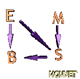 network construction and inference is in order. Suppose we have a simple domain, consisting of a population of people, their bank account (B=credit,debt), their employment status (E=job,unemp), their money management (M=good,bad) abilities and their spending habits (S=spend,thrift). We could build a belief network which looks like figure MONNET. Their
bank account depends on whether they are paid, and whether they spend much, and their spending depends on how much money they have, how much time they have and whether they are careful not to go into debt. Undoubtedly this is a very noddy example, and real life belief networks will be larger and more complicated.
network construction and inference is in order. Suppose we have a simple domain, consisting of a population of people, their bank account (B=credit,debt), their employment status (E=job,unemp), their money management (M=good,bad) abilities and their spending habits (S=spend,thrift). We could build a belief network which looks like figure MONNET. Their
bank account depends on whether they are paid, and whether they spend much, and their spending depends on how much money they have, how much time they have and whether they are careful not to go into debt. Undoubtedly this is a very noddy example, and real life belief networks will be larger and more complicated.
Of course a belief network alone is not good enough, we need some numbers too. We might choose the following conditional probability tables (CPTs) as being reasonably representative of those probabilities. In real life situations we would probably want to tune or learn these CPTs based on historical examples.
| P(E=job) | P(E=unemp) | P(M=good) | P(M=bad) |
| 0.9 | 0.1 | 0.6 | 0.4 |
| E | M | P(S=spend) | P(S=thrift) |
| job | good | 0.5 | 0.5 |
| job | bad | 0.9 | 0.1 |
| unemp | good | 0.2 | 0.8 |
| unemp | bad | 0.7 | 0.3 |
| E | S | P(B=credit) | P(B=debt) |
| job | spend | 0.6 | 0.4 |
| job | thrift | 1.0 | 0.0 |
| unemp | spend | 0.2 | 0.8 |
| unemp | thrift | 0.6 | 0.4 |
These tables specify all the conditional probabilities that are needed. Belief network construction is finished.
This leads to the topic of this section. Inference is modifying beliefs in light of evidence. Suppose we know that a person is in debt, and has been spending a lot of money. We might want to know whether or not they have a job. We are interested in the posterior probability P(E|B=debt,S=spend). To calculate this probability we first calculate P(E,M|B=debt,S=spend). This is proportional to P(B|E,S)P(S|E,M)P(E)P(M) by simple application of probability theory (in fact using Bayes rule). Plugging in the numbers from each of the tables (looking at the B=debt,S=spend columns/rows), and normalising so that the probabilities sum to one to account for the constant of proportionality, we get
| E | M | P(B|E,S)P(S|E,M)P(E)P(M) | P(E,M|B=debt,S=spend) |
| job | good | 0.4x0.5x0.9x0.6=0.11 | 0.40 |
| job | bad | 0.4x0.9x0.9x0.4=0.13 | 0.48 |
| unemp | good | 0.8x0.2x0.1x0.6=0.010 | 0.04 |
| unemp | bad | 0.8x0.7x0.1x0.4=0.022 | 0.08 |
where we have rounded to a couple of decimal places. To find P(E|B=debt,S=spend) we have to sum over all the possible values that M takes. This gives the final result
| P(E=job|B=debt,S=spend) | P(E=unemp|B=debt,S=spend) |
| 0.88 | 0.12 |
From this table we can see that the probability of the person being unemployed goes up a little (from 0.1 to 0.12) in light of the information we have. If on the other had we had asked about their money management skills we would get
| P(M=good|B=debt,S=spend) | P(M=bad|B=debt,S=spend) |
| 0.44 | 0.56 |
In other words we would get a more significant change (from 0.4 to 0.56) in the probability that they had poor money management skills.
Hopefully this has illustrated what is meant by inference in belief networks. An example like this is particularly useless in practice because a) the number of variables and states is too small making the network oversimple for the task at hand, and b) because I plucked the numbers out of thin air! Subject a) is the topic of the next section, and b) is the subject of the following section on learning in belief networks.
Exact and Approximate Inference
One situation when belief network inference is straightforward is in singly connected networks. A singly connected network is a graph where there is only one undirected path from any node to any other node (in an undirected path the arrow directions are ignored). In this situation there is a simple approach to solving the inference problem which is called belief propagation.
Consider a tree structured network, which is a basic sort of simply connected graphical model. If we want to condition on certain nodes of this tree structured network, it does not introduce serious problems. This is because conditioning on a node splits the network into two parts, the descendants of the conditioned node, and the remainder of the network. In each of these parts the new information at the conditioned nodes effects the nodes which it is directly connected to. These in turn effect the nodes they are connected to and so on. Because there are no loops in the network, it is possible to follow the chain of effect until all the nodes are reached once and only once. It turns out that there is a simple way to propagate beliefs through these networks in order to obtain the updated probabilities. This is called belief propagation due to Pearl [1988]. It involves passing a set of messages up the tree from the conditioned nodes (called the lambda messages, and analogous to likelihoods), and then a further set of messages down the tree (called pi messages and analogous to priors). The final posterior marginal probabilities at the nodes are proportional to the product of the lambda and pi messages at each of the nodes. (In fact the whole posterior distribution can be reconstructed from this information as the belief network of the posterior is a set of disjoint trees). I will not duplicate the belief propagation algorithm and theory here, as it is available in many places.
On the other hand there are many situations in which networks are not tree structured. Sometimes it is possible to use generalisations of belief propagation, such as the junction tree algorithm, but quite often it is necessary to resort to approximation methods. Two popular approaches include sampling and variational methods. The sampling approach involves constructing a Markov chain which has the desired posterior as the limit distribution. Samples from this Markov chain are used as an approximation for the posterior. The variational approach, on the other hand, fits an approximating distribution to the true posterior. The variational distribution must be chosen to be tractable to calculate with and must allow a variational fit to the posterior to be obtained in a reasonable time. At the same time the fit must be as good as possible so that the approximation is not a poor one. This makes choosing the variational distribution a non-trivial exercise.
Learning and the EM algorithm
The final issue which will be considered here involves the question about how to set or learn the conditional probabilities in our belief network. In practice these are often learnt from past data. In fact learning the conditional probability parameters of a belief network is another example of Bayesian inference, just inference at a higher level: we are inferring the value of the parameters using a whole set of data which are all understood to be potentially generated from a network with one set of parameters.
In order to learn the values of the parameters, we need to have some prior distribution over the values the parameters can take. This could be a broad and unrestrictive distribution, expressing little knowledge in the values which the conditional probabilities take. Then we need some approach to using the data to calculate the posterior probability of the parameters.
The EM algorithm is a common approach for learning in belief networks. In its standard form it cheats a little as it does not calculate the full posterior probability distribution of the parameters, but rather focusses in on the maximum a posteriori parameter values. Given the problem is a hard one, this is a reasonable start.
The EM algorithm works by taking an iterative approach to inference an learning. In the first step, called the E step, the EM algorithm performs inference in the belief network for each of the datum in the dataset. This allows the information from the data to be used, and various necessary statistics S to be calculated from the resulting posterior probabilities. Then in the M step, parameters are chosen to maximise the log posterior logP(T|D,S) given these statistics are fixed. Of course the result is that we now have a new set of parameters, with the result that the statistics S which we collected are no longer accurate. Hence the E step must be repeated, then the M step and so on. At each stage the EM algorithm guarantees that the posterior probability must increase. Hence it eventually converges to a local maxima of the log posterior.
This is one way in which conditional probabilities can be learnt from historic data. Having learnt the conditional probabilities these can now be used in the network to make predictions for future data. Hence we have a structured and principled approach for making predictions using a combination of prior knowledge and past data. It is this powerful combination which makes belief networks such a versatile tool.
Conclusions
Belief Networks are a very general tool in Bayesian statistics. Their combination of structural characteristics with probability theory allows large probability distributions to be handled and manipulated which otherwise would be very cumbersome. Considering belief network structure also allows suitable algorithms for inference to be developed. There is little doubt that the applications of belief networks will continue to grow widely. The purpose of this tutorial is to give a quick and basic and simple introduction to the motivation and inner workings of belief network methods.
A Few References
There are many good places to look for references on belief networks. For a solid technical introduction and development of exact inference in belief networks, see
- Castillo, E., J. M. Gutierrez and A. S. Hadi (1997) Expert systems and probabilistic network models. Springer-Verlag.
Pearls orginal book is still worth a read, and introduces the concepts well.
- Pearl, J. (1988) Probabilistic Reasoning in Intelligent Systems: Networks of Plausible Inference. Morgan Kaufmann.
Looking at learning, Jordan edited a collection of papers:
- Jordan, M.I. ed (1998) Learning in Graphical Models. MIT Press.
and Heckerman has a good tutorial:
- Heckerman, D. (1996) A tutorial on learning with Bayesian networks, Microsoft Research tech. report, MSR-TR-95-06.
Variational Inference and MonteCarlo methods are described in
- Jordan, M.I., Z. Ghahramani, T. S. Jaakkola, and L. K. Saul (1998) An introduction to variational methods for graphical models
and
- MacKay, D. (1998) An introduction to Monte Carlo methods.
There are many, many more excellent books and papers which are referred to in these publications.