Amos Storkey


The introduction of non-stationarity into the Gaussian process framework can be straightforward. Sometimes the non-stationarity is simply an additive mean. Not all non-stationarities can be treated that way though: it might be that given the means, the covariance function still changes from one part of the space to another. Modelling these types of processes requires a different approach.
Sometimes we might know apriori the non-stationary covariance structure. If this is the case then the Gaussian process treatment can be used without modification. We simply have a position dependent covariance function, and calculate the covariance matrix between two points from their absolute rather than relative po sitions.
This situation is rarely the case. Often we might know exactly the nature of the non-stationarity. In these situations we can follow a sampling procedure. We can draw up a model representing the different possible non-stationary covariance structures. Then we can sample from these models to choose a single model, from which an exact covariance function can be calculated. When a number of these samples are collected the final integration over all possible models of the non-stationarity can be approx imated by the relevant sample sum.
There is a catch to this method though. Each sample corresponds to a distinctly different covariance matrix. As a result a matrix inverse has to be calculated for each sample, at great computational expense. This can become a significant problem if it takes some time to explore the sample space and to settle to an equilibrium distribution.
Very often the data under study has not been generated from a stationary process. A common example of this is where a
number of different signal sources are present, and the observable signal is created by switching between these different regimes.
In this problem, it is believed that there are a fixed number of source signals.
It is on the whole assumed that these
signals are independent. The measured signal, however, only has information from any one of the signals at any one
time. In other words at any point the measured signal can be seen to be created
by a signal chosen from the set of
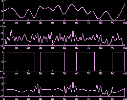
sources by some discrete random process. The figure below illustrates
this. The top two graphs are two
independent sources. The third graph illustrates the switching process. The final graph gives the final signal made up
of parts of each of the two sources.
 Hence the resulting signal is made up of different regimes, each of
which gives the state of one of the source signals.
Hence the resulting signal is made up of different regimes, each of
which gives the state of one of the source signals.
This situation can be modelled with a mixture of Gaussian processes in the way that has been described above. Latent variables represent which of the current regimes generated a sample datum. Then different hyperparameters or covariance structures can be used to represent the characteristics of the different regimes. The great benefit of Gaussian processes is that the covariance matrix structure can represent many different signal structures and textures, from smooth curves to random fractal textures.
As it is not known which regime is generating the signal at any point, and the structure of the signals is unknown, these variables/parameters are given prior distributions which should be integrated over.
| Contents || Introduction || Background || Research || Group || Publications|| Demonstrations || Teaching || Interests || Links || Contact || email |
| © Amos Storkey 2000-2004. |