Surface images are an iconic representation similar in structure to traditional intensity images, except that they record surface properties, such as absolute depth and surface orientation in the camera coordinate system. The positional relationship between the scene and the image is described by projective geometry. In this way, surface images are a subset of intrinsic images [20], except that here the information is solely related to the surface shape, and not to reflectance. This eliminates surface markings, shadows, highlights, image flow, shading and other illumination and observer dependent effects from the information (which are also important, but are not considered here).
A second similar representation is Marr's
![]() sketch [112].
This represents mainly surface orientation, depth and
labeled boundaries with region groupings.
As his work was unfinished, there is controversy over the precise details
of his proposal.
sketch [112].
This represents mainly surface orientation, depth and
labeled boundaries with region groupings.
As his work was unfinished, there is controversy over the precise details
of his proposal.
There are several forms of redundancy in this information (e.g. surface
orientation is
derivable from distance), but here we are more concerned with how to use
the information than how it was acquired or how to make it robust.
Segmentation
The surface image is segmented into significant regions, resulting in a set of connected boundary segments that partition the whole surface image. What "significant" means has not been agreed on (e.g. [166,107]), and little has been written on it in the context of surface representations. For the purposes of this research, it means surface image regions corresponding to connected object surface regions with approximately uniform curvature and not otherwise terminated by a surface shape discontinuity. Here, "uniform curvature" means that the principal curvatures are nearly constant over the region. The goal of this segmentation is to produce uniform regions whose shape can be directly compared to that of model SURFACEs.
The proposed criteria that cause this segmentation are:
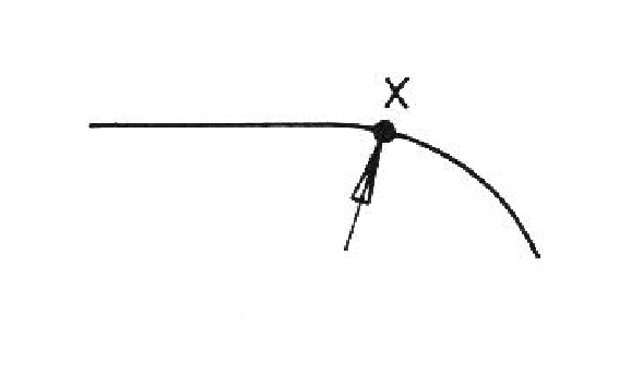
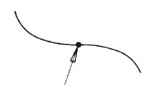
These four criteria are probably just minimum constraints. The first rule is obvious because, at a given scale, surface portions separated by depth should not be in the same segment. The second rule applies at folds in surfaces or where two surfaces join. Intuitively, the two sections are considered separate surfaces, so they should be segmented. The third and fourth rules are less intuitive and are illustrated in Figures 3.1 and 3.2. The first example shows a cross section of a planar surface changing into a uniformly curved one. Neither of the first two rules applies, but a segmentation near point X is clearly desired. However, it is not clear what should be done when the curvature changes continuously. Figure 3.2 shows a change in the curvature direction vector that causes segmentation as given by the fourth rule. Descriptions D, C1, C2m and C2d are sensitive to changes in scale and description D depends on the observer's position.
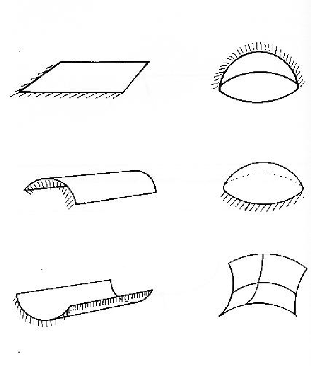
These criteria segment surfaces into patches of the six classes illustrated in Figure 3.3. The class labels can then be used as symbolic descriptions of the surface.
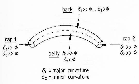
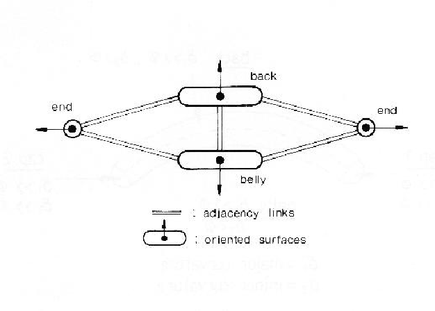
Figure 3.4 shows the segmentation of a sausage image. The segmentation produces four object surfaces (two hemispherical ends, a nearly cylindrical "back", and a saddle surface "belly") plus the background planar surface. The segmentation between the back and belly occurs because the surface changes from ellipsoidal to hyperboloidal. These segments are stable to minor changes in the sausage's shape (assuming the same scale of analysis is maintained), and are members of the six surface classes. Figure 3.10 shows the surface patches produced by the segmentation criteria for the test scene.
The segmented sausage can be represented by the graph of Figure 3.5. Here, the nodes represent the surfaces and are labeled by the surface class, curvature values and nominal orientations. The links denote adjacency.
The theoretical grounds for these conditions and how to achieve them are not settled, but the following general principles seem reasonable. The segmentation should produce connected regions of constant character with all curvature magnitudes roughly the same and in the same direction. Further, the segmentations should be stable to viewpoint and minor variations in object shape, and should result in unique segmentations. Because the criteria are object-centered, they give unique segmentation, independent of viewpoint. As we can also apply the criteria to the models, model invocation (Chapter 8) and matching (Chapter 9) are simplified by comparing similar corresponding features. The examples used in this book were chosen to be easily and obviously segmentable to avoid controversy. Thus, image and model segmentations will have roughly corresponding surface regions, though precisely corresponding boundaries are not required.
Scale affects segmentation because some shape variations are insignificant when compared to the size of objects considered. In particular, less pronounced shape segmentations will disappear into insignificance as the scale of analysis grows. No absolute segmentation boundaries exist on free-form objects, so criteria for a reasonable segmentation are difficult to formulate. (Witkin [165] has suggested a stability criterion for scale-based segmentations of one dimensional signals.)
This does not imply that the segmentation boundaries must remain constant. For some ranges of scale, the sausage's boundaries (Figure 3.4) will move slightly, but this will not introduce a new segmented surface. Invocation and matching avoid the boundary movement effects by emphasizing the spatial relationships between surfaces (e.g. adjacency and relative orientation) and not the position of intervening boundaries.
Some research into surface segmentation has occurred. Brady et al. [40] investigated curvature-based local descriptions of curved surfaces, by constructing global features (i.e. regions and lines of curvature) from local properties (i.e. local principal curvatures). Besl [24] started with similar curvature properties to seed regions, but then used numerical techniques to fit surface models to the data (e.g. to ellipsoidal patches) and grow larger patches. This work was particularly effective. Hoffman and Jain [90] clustered surface normals to produce three types of patches (planar, convex and concave). Patches were linked by four types of boundary (depth discontinuity, orientation discontinuity, tesselation and null). Null and tesselation boundaries were later removed to produce larger patches.
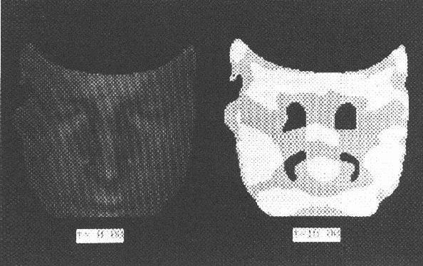
Following on from Besl's work, Cai [43] has been investigating multiple scale segmentation of surface patches from range data. He used a modified diffusion smoothing process to blend the features and then forms surface patches from region growing based on local principal curvature estimates. Large features that remain over several scales are selected to form a stable representation. Figure 3.6 shows an intermediate stage of the segmentation of a face, where the positive ellipsoidal regions are shown in white, hyperboloidal regions are grey and negative ellipsoidal regions are black. Though there is still considerable research on segmentation to be done, features such as these are suitable for recognition with a coarse scale model.
With the segmentation processes described above, the boundary labeling problem becomes trivial. The purpose of the labeling is to designate which boundaries result from the shape segmentations, and which result from occlusion. The type of a shape segmentation boundary is probably not important, as scale affects the labeling, so it is not used. However, the different types are recorded for completeness and the shape of the boundary helps to identify particular surfaces.
Occlusion boundaries are further distinguished into the boundary
lying on a closer obscuring surface and that lying on a distant
surface.
All shape discontinuity boundaries are labeled as convex, concave or crack.
Inputs Used in the Research
Because the geometry of the surface image is the same as that of an intensity image, an intensity image was used to prepare the initial input. From this image, all relevant surface regions and labeled boundaries were extracted, by hand, according to the criteria described previously. The geometry of the segmenting boundaries was maintained by using a registered intensity image as the template. Then, the distances to and surface orientations of key surface points were recorded at the corresponding pixel. The labeled boundaries and measured points were the inputs into the processes described in this book.
The surface orientation was recorded for each measured point, and a single measurement point was sufficient for planar surfaces. For curved surfaces, several points (6 to 15) were used to estimate the curvature, but it turned out that not many were needed to give acceptable results. As the measurements were made by hand, the angular accuracy was about 0.1 radian and distance accuracy about 1 centimeter.
Those processes that used the surface information directly (e.g. for computing
surface curvature) assumed that the distance and orientation information
was dense over the whole image.
Dense data values were interpolated from values of nearby measured points,
using a ![]() image distance weighting.
This tended to flatten the interpolated surface in the region of the data
points, but had the
benefit of emphasizing data points closest to the test point.
A surface approximation approach (e.g. [77]) would have been better.
The interpolation used only those points from within the segmented surface
region, which was appropriate because the regions were selected for
having uniform curvature class.
image distance weighting.
This tended to flatten the interpolated surface in the region of the data
points, but had the
benefit of emphasizing data points closest to the test point.
A surface approximation approach (e.g. [77]) would have been better.
The interpolation used only those points from within the segmented surface
region, which was appropriate because the regions were selected for
having uniform curvature class.
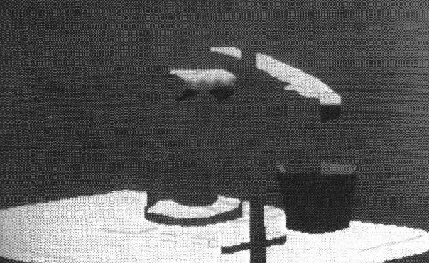
We now show the input data for the test scene in greater
detail.
Figure 1.1 showed the original test scene and
Figure 1.4 showed the depth information coded so dark means further
away.
Figure 3.7 shows the ![]() component of the unit surface normal.
Here, brighter means more upward facing.
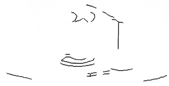
Figure 1.5 showed the occlusion label boundaries.
Figure 3.8 shows the
orientation discontinuity label boundaries and Figure 3.9
shows the curvature discontinuity boundary.
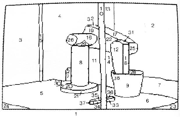
Figure 3.10 shows the identifier assigned to each region and
the overall segmentation boundaries.
component of the unit surface normal.
Here, brighter means more upward facing.
Figure 1.5 showed the occlusion label boundaries.
Figure 3.8 shows the
orientation discontinuity label boundaries and Figure 3.9
shows the curvature discontinuity boundary.
Figure 3.10 shows the identifier assigned to each region and
the overall segmentation boundaries.
The labeled, segmented surface image was represented as a graph, because it was compact and easily exploited key structural properties of the data. These are:
The computation that makes this transformation is a trivial boundary tracking and graph linking process. No information is lost in the transformations between representations, because of explicit linking back to the input data structures (even if there is some loss of information in the generalization at any particular level). The only interesting point is that before tracking, the original segmented surface image may need to be preprocessed. The original image may have large gaps between identified surface regions. Before boundary tracking, these gaps have to be shrunk to single pixel boundaries, with corresponding region extensions. (These extensions have surface orientation information deleted to prevent conflicts when crossing the surface boundaries.) This action was not needed for the hand segmented test cases in this research.