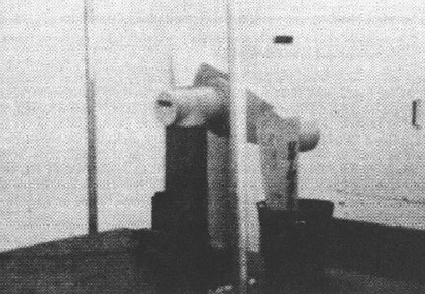
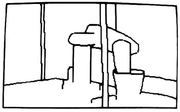
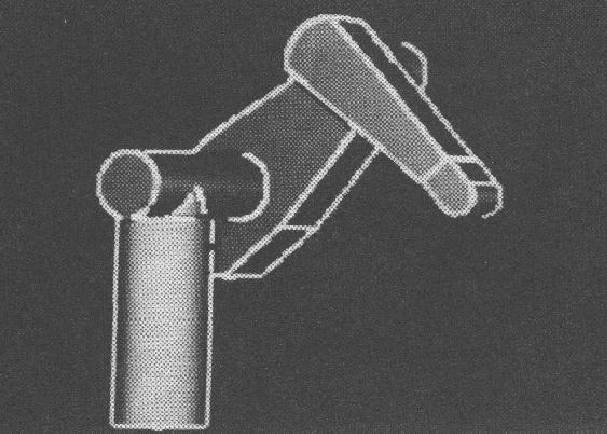
This section summarizes the work discussed in the rest of the book by presenting an example of IMAGINE I's surface-based object recognition [68]. The test image discussed in the following example is shown in Figure 1.1. The key features of the scene include:
Recognition is based on comparing observed and deduced properties with those of a prototypical model. This definition immediately introduces five subtasks for the complete recognition process:
The deduction process needs the location and orientation of the object to predict obscured structures and their properties, so this adds:
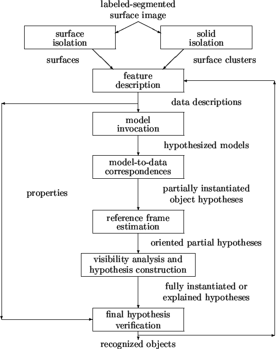
The remainder of this section elaborates on the processes and the data flow dependencies that constrain their mutual relationship in the complete recognition computation context. Figure 1.2 shows the process sequence determined by the constraints, and is discussed in more detail below.
Recognition starts from surface data, as represented in a structure
called a labeled, segmented surface image (Chapter 3).
This structure is like Marr's
![]() sketch and includes a pointillistic
representation of absolute depth and local surface orientation.
sketch and includes a pointillistic
representation of absolute depth and local surface orientation.
Data segmentation and organization are both difficult and important. Their primary justifications are that segmentation highlights the relevant features for the rest of the recognition process and organization produces, in a sense, a figure/ground separation. Properties between unrelated structure should not be computed, such as the angle between surface patches on separate objects. Otherwise, coincidences will invoke and possibly substantiate non-existent objects. Here, the raw data is segmented into regions by boundary segments labeled as shape or obscuring. Shape segmentation is based on orientation, curvature magnitude and curvature direction discontinuities. Obscuring boundaries are placed at depth discontinuities. These criteria segment the surface image into regions of nearly uniform shape, characterized by the two principal curvatures and the surface boundary. As no fully developed processes produce this data yet, the example input is from a computer augmented, hand-segmented test image. The segmentation boundaries were found by hand and the depth and orientation values were interpolated within each region from a few measured values.
The inputs used to analyze the test scene shown in Figure
1.1 are shown in Figures 1.3 to 1.6.
Figure 1.3 shows the depth values associated with the scene, where the lighter
values mean closer points.
Figure 1.4 shows the cosine of the surface slant for each image point.
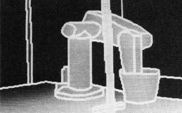
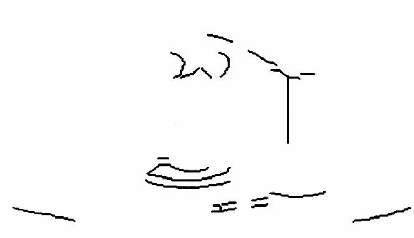
Figure 1.5 shows the obscuring boundaries.
Figure 1.6 shows the shape segmentation boundaries.
From these pictures, one can get the general impression of the rich data
available and the three dimensional character of the scene.
Complete Surface Hypotheses
Image segmentation leads directly to partial or complete object surface segments. Surface completion processes (Chapter 4) reconstruct obscured portions of surfaces, when possible, by connecting extrapolated surface boundaries behind obscuring surfaces. The advantage of this is twofold: it provides data surfaces more like the original object surface for property extraction and gives better image evidence during hypothesis construction. Two processes are used for completing surface hypotheses. The first bridges gaps in single surfaces and the second links two separated surface patches. Merged surface segments must have roughly the same depth, orientation and surface characterization. Because the reconstruction is based on three dimensional surface image data, it is more reliable than previous work that used only two dimensional image boundaries. Figure 1.7 illustrates both rules in showing the original and reconstructed robot upper arm large surface from the test image.
Surface hypotheses are joined to form surface clusters, which are blob-like three dimensional object-centered representations (Chapter 5). The goal of this process is to partition the scene into a set of three dimensional solids, without yet knowing their identities. Surface clusters are useful (here) for aggregating image features into contexts for model invocation and matching. They would also be useful for tasks where identity is not necessary, such as collision avoidance.
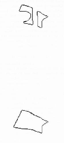
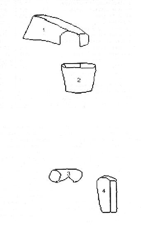
A surface cluster is formed by finding closed loops of isolating boundary segments. The goal of this process is to create a blob-like solid that encompasses all and only the features associated with a single object. This strengthens the evidence accumulation used in model invocation and limits combinatorial matching during hypothesis construction. Obscuring and concave surface orientation discontinuity boundaries generally isolate solids, but an exception is for laminar objects, where the obscuring boundary across the front lip of the trash can (Figure 1.8) does not isolate the surfaces. These criteria determine the primitive surface clusters. A hierarchy of larger surface clusters are formed from equivalent depth and depth merged surface clusters, based on depth ordering relationships. They become larger contexts within which partially self-obscured structure or subcomponents can be found. Figure 1.8 shows some of the primitive surface clusters for the test scene. The clusters correspond directly to primitive model ASSEMBLYs (which represent complete object models).
General identity-independent properties (Chapter 6) are used to drive the invocation process to suggest object identities, which trigger the model-directed matching processes. Later, these properties are used to ensure that model-to-data surface pairings are correct. The use of three dimensional information from the surface image makes it possible to compute many object properties directly (as compared to computing them from a two dimensional projection of three dimensional data).
This task uses the surfaces and surface clusters produced by the segmentation
processes.
Surface and boundary shapes are the key properties for surfaces.
Relative feature sizes, spatial relationships and adjacency are the
properties needed for solid recognition.
Most of the measured properties relate to surface patches and include:
local curvature, absolute area, elongation and surface intersection
angles.
As an example, Table 1.1 lists the estimated properties for the
robot shoulder circular end panel (region 26 in Figure 3.10).
| PROPERTY | ESTIMATED | TRUE |
|---|---|---|
| maximum surface curvature | 0.0 | 0.0 |
| minimum surface curvature | 0.0 | 0.0 |
| absolute area | 165 | 201 |
| relative area | 0.24 | 0.25 |
| surface size eccentricity | 1.4 | 1.0 |
| adjacent surface angle | 1.47 | 1.57 |
| number of parallel boundaries | 1 | 1 |
| boundary curve length | 22.5 | 25.1 |
| boundary curve length | 25.3 | 25.1 |
| boundary curvature | 0.145 | 0.125 |
| boundary curvature | 0.141 | 0.125 |
| number of straight segments | 0 | 0 |
| number of arc segments | 2 | 2 |
| number of equal segments | 1 | 1 |
| number of right angles | 0 | 0 |
| boundary relative orientation | 3.14 | 3.14 |
| boundary relative orientation | 3.14 | 3.14 |
The modeled objects (Chapter 7) are compact, connected solids with definable shapes, where the complete surfaces are rigid and segmentable into regions of constant local shape. The objects may also have subcomponents joined by interconnections with degrees-of-freedom.
Identification requires known object representations with three components: a geometric model, constraints on object properties, and a set of inter-object relationships.
The SURFACE patch is the model primitive, because surfaces are the primary data units. This allows direct pairing of data with models, comparison of surface shapes and estimation of model-to-data transformation parameters. SURFACEs are described by their principal curvatures with zero, one or two curvature axes, and by their extent (i.e. boundary). The segmentation ensures that the shape (e.g. principal curvatures) remains relatively constant over the entire SURFACE.
Larger objects (called ASSEMBLYs) are recursively constructed from SURFACEs or other ASSEMBLYs using coordinate reference frame transformations. Each structure has its own local reference frame and larger structures are constructed by placing the subcomponents in the reference frame of the aggregate. Partially constrained transformations can connect subcomponents by using variables in the attachment relationship. This was used for the PUMA robot's joints. The geometric relationship between structures is useful for making model-to-data assignments and for providing the adjacency and relative placement information used by verification.
The three major object models used in this analysis are the PUMA robot, chair and trash can. (These models required the definition of 25 SURFACEs and 14 ASSEMBLYs.) A portion of the robot model definition is shown below.
Illustrated first is the SURFACE definition for the robot upper arm large curved end panel (uendb). The first triple on each line gives the starting endpoint for a boundary segment. The last item describes the segment as a LINE or a CURVE (with its parameters in brackets). PO means the segmentation point is a boundary orientation discontinuity point and BO means the boundary occurs at an orientation discontinuity between the surfaces. The next to last line describes the surface type with its axis of curvature and radii. The final line gives the surface normal at a nominal point in the SURFACE's reference frame.
SURFACE uendb =
    PO/(0,0,0) BO/LINE
    PO/(10,0,0) BO/CURVE[0,0,-22.42]
    PO/(10,29.8,0) BO/LINE
    PO/(0,29.8,0) BO/CURVE[0,0,-22.42]
    CYLINDER [(0,14.9,16.75),(10,14.9,16.75),22.42,22.42]
    NORMAL AT (5,15,-5.67) = (0,0,-1);
Illustrated next is the rigid upperarm ASSEMBLY with its SURFACEs
(e.g. uendb) and the reference frame relationships
between them.
The first triple in the relationship is the (![]() ,
, ![]() ,
, ![]() ) translation and the
second gives the (rotation, slant, tilt) rotation.
Translation is applied after rotation.
) translation and the
second gives the (rotation, slant, tilt) rotation.
Translation is applied after rotation.
ASSEMBLY upperarm\= =
    uside AT ((-17,-14.9,-10),(0,0,0))
    uside AT ((-17,14.9,0),(0,pi,pi/2))
    uendb AT ((-17,-14.9,0),(0,pi/2,pi))
    uends AT ((44.8,-7.5,-10),(0,pi/2,0))
    uedges AT ((-17,-14.9,0),(0,pi/2,3*pi/2))
    uedges AT ((-17,14.9,-10),(0,pi/2,pi/2))
    uedgeb AT ((2.6,-14.9,0),(0.173,pi/2,3*pi/2))
    uedgeb AT ((2.6,14.9,-10),(6.11,pi/2,pi/2));
The ASSEMBLY that pairs the upper and lower arm rigid structures into a non-rigidly connected structure is defined now. Here, the lower arm has an affixment parameter that defines the joint angle in the ASSEMBLY.
ASSEMBLY armasm =
    upperarm AT ((0,0,0),(0,0,0))
    lowerarm AT ((43.5,0,0),(0,0,0))
    FLEX ((0,0,0),(jnt3,0,0));
Figure 1.9 shows an image of the whole robot ASSEMBLY with the surfaces shaded according to surface orientation.
Property constraints are the basis for direct evidence in the model invocation process and for identity verification. These constraints give the tolerances on properties associated with the structures, and the importance of the property in contributing towards invocation. Some of the constraints associated with the robot shoulder end panel named "robshldend" are given below (slightly re-written from the model form for readability). The first constraint says that the relative area of the robshldend in the context of a surface cluster (i.e. the robot shoulder) should lie between 11% and 40% with a peak value of 25%, and the weighting of any evidence meeting this constraint is 0.5.
    UNARYEVID 0.11\  < relative_area < 0.40 PEAK 0.25 WEIGHT 0.5;
    UNARYEVID 156.0 < absolute_area < 248.0 PEAK 201.0 WEIGHT 0.5;
    UNARYEVID 0.9 < elongation < 1.5 PEAK 1.0 WEIGHT 0.5;
    UNARYEVID 0 < parallel_boundary_segments < 2 PEAK 1 WEIGHT 0.3;
    UNARYEVID 20.1 < boundary_length < 40.0 PEAK 25.1 WEIGHT 0.5;
    UNARYEVID .08 < boundary_curvature < .15 PEAK .125 WEIGHT 0.5;
    BINARYEVID 3.04 < boundary_relative_orientation(edge1,edge2) < 3.24 PEAK 3.14 WEIGHT 0.5;
Rather than specifying all of an object's properties, it is possible to specify some descriptive attributes, such as "flat". This means that the so-described object is an instance of type "flat" - that is, "surfaces without curvature". There is a hierarchy of such descriptions: the description "circle" given below is a specialization of "flat". For robshldend, there are two descriptions: circular, and that it meets other surfaces at right angles:
    DESCRIPTION OF robshldend IS circle 3.0;
    DESCRIPTION OF robshldend IS sapiby2b 1.0;
Relationships between objects define a network used to accumulate invocation evidence. Between each pair of model structures, seven types of relationship may occur: subcomponent, supercomponent, subclass, superclass, descriptive, general association and inhibition. The model base defines those that are significant to each model by listing the related models, the type of relationship and the strength of association. The other relationship for robshldend is:
SUPERCOMPONENT OF robshldend IS robshldbd 0.10;
Evidence for subcomponents comes in visibility groups (i.e. subsets of all object features), because typically only a few of an object's features are visible from any particular viewpoint. While they could be deduced computationally (at great expense), the visibility groups are given explicitly here. The upperarm ASSEMBLY has two distinguished views, differing by whether the big (uendb) or small (uends) curved end section is seen.
    SUBCGRP OF upperarm = uside uends uedgeb uedges;
    SUBCGRP OF upperarm = uside uendb uedgeb uedges;
Model Invocation
Model invocation (Chapter 8) links the identity-independent processing to the model-directed processing by selecting candidate models for further consideration. It is essential because of the impossibility of selecting the correct model by sequential direct comparison with all known objects. These models have to be selected through suggestion because: (a) exact individual models may not exist (object variation or generic description) and (b) object flaws, sensor noise and data loss lead to inexact model-to-data matchings.
Model invocation is the purest embodiment of recognition - the inference of identity. Its outputs depend on its inputs, but need not be verified or verifiable for the visual system to report results. Because we are interested in precise object recognition here, what follows after invocation is merely verification of the proposed hypothesis: the finding of evidence and ensuring of consistency.
Invocation is based on plausibility, rather than certainty, and this notion is expressed through accumulating various types of evidence for objects in an associative network. When the plausibility of a structure having a given identity is high enough, a model is invoked.
Plausibility accumulates from property and relationship evidence, which allows graceful degradation from erroneous data. Property evidence is obtained when data properties satisfy the model evidence constraints. Each relevant description contributes direct evidence in proportion to a weight factor (emphasizing its importance) and the degree that the evidence fits the constraints. When the data values from Table 1.1 are associated with the evidence constraints given above, the resulting property evidence plausibility for the robshldend panel is 0.57 in the range [-1,1].
Relationship evidence arises from conceptual associations with other structures and identifications. In the test scene, the most important relationships are supercomponent and subcomponent, because of the structured nature of the objects. Generic descriptions are also used: robshldend is also a "circle". Inhibitory evidence comes from competing identities. The modeled relationships for robshldend were given above. The evidence for the robshldend model was:
Plausibility is only associated with the model being considered and a context; otherwise, models would be invoked for unlikely structures. In other words, invocation must localize its actions to some context inside which all relevant data and structure must be found. The evidence for these structures accumulates within a context appropriate to the type of structure:
The invocation computation accumulates plausibility in
a relational network
of {context} ![]() {identity} nodes
linked to each other by relationship arcs and linked to
the data by the property constraints.
The lower level nodes in this network are general
object structures, such as planes, positive cylinders
or right angle surface junctions.
From these, higher level object structures are linked hierarchically.
In this way, plausibility accumulates upwardly from simple to more
complex structures.
This structuring provides both richness in discrimination through
added detail, and efficiency of association (i.e. a structure
need link only to the most compact levels of subdescription).
Though every model must ultimately be a candidate for every
image structure, the network formulation achieves efficiency through
judicious selection of appropriate conceptual units and
computing plausibility over the entire network in parallel.
{identity} nodes
linked to each other by relationship arcs and linked to
the data by the property constraints.
The lower level nodes in this network are general
object structures, such as planes, positive cylinders
or right angle surface junctions.
From these, higher level object structures are linked hierarchically.
In this way, plausibility accumulates upwardly from simple to more
complex structures.
This structuring provides both richness in discrimination through
added detail, and efficiency of association (i.e. a structure
need link only to the most compact levels of subdescription).
Though every model must ultimately be a candidate for every
image structure, the network formulation achieves efficiency through
judicious selection of appropriate conceptual units and
computing plausibility over the entire network in parallel.
When applied to the full test scene, invocation was generally successful.
There were 21 SURFACE invocations of 475 possible, of
which 10 were correct, 5 were justified because of similarity and 6
were unjustified.
There were 18 ASSEMBLY invocations of 288 possible, of which 10 were
correct, 3 were justified because of similarity and 5 were unjustified.
Hypothesis Construction
Hypothesis construction (Chapter 9) aims for full object recognition, by finding evidence for all model features. Invocation provides the model-to-data correspondences to form the initial hypothesis. Invocation thus eliminates most substructure search by directly pairing features. SURFACE correspondences are immediate because there is only one type of data element - the surface. Solid correspondences are also trivial because the matched substructures (SURFACEs or previously recognized ASSEMBLYs) are also typed and are generally unique within the particular model. All other data must come from within the local surface cluster context.
The estimation of the ASSEMBLY and SURFACE reference frames is one goal of hypothesis construction. The position estimate can then be used for making detailed metrical predictions during feature detection and occlusion analysis (below).
Object orientation is estimated by transforming the nominal orientations of pairs of model surface vectors to corresponding image surface vectors. Pairs are used because a single vector allows a remaining degree of rotational freedom. Surface normals and curvature axes are the two types of surface vectors used. Translation is estimated from matching oriented model SURFACEs to image displacements and depth data. The spatial relationships between structures are constrained by the geometric relationships of the model and inconsistent results imply an inappropriate invocation or feature pairing.
Because of data errors, the six degrees of spatial freedom are represented as parameter ranges. Each new model-to-data feature pairing contributes new spatial information, which helps further constrain the parameter range. Previously recognized substructures also constrain object position.
The robot's position and joint angle estimates were also found using a geometric reasoning network approach [74]. Based partly on the SUP/INF methods used in ACRONYM [42], algebraic inequalities that defined the relationships between model and data feature positions were used to compile a value-passing network. The network calculated upper and lower bounds on the (e.g.) position values by propagating calculated values through the network. This resulted in tighter position and joint angle estimates than achieved by the vector pairing approach.
Table 1.2 lists the measured and estimated location positions,
orientations and joint angles for the robot.
The test data was obtained from about 500 centimeters distance.
| PARAMETER | MEASURED | ESTIMATED |
|---|---|---|
| X | 488 (cm) | 487 (cm) |
| Y | 89 (cm) | 87 (cm) |
| Z | 554 (cm) | 550 (cm) |
| Rotation | 0.0 (rad) | 0.04 (rad) |
| Slant | 0.793 (rad) | 0.70 (rad) |
| Tilt | 3.14 (rad) | 2.97 (rad) |
| Joint 1 | 2.24 (rad) | 2.21 (rad) |
| Joint 2 | 2.82 (rad) | 2.88 (rad) |
| Joint 3 | 4.94 (rad) | 4.57 (rad) |
Once position is estimated, a variety of model-driven processes contribute to completing an oriented hypothesis. They are, in order:
Hypothesis construction has a "hierarchical synthesis" character, where data surfaces are paired with model SURFACEs, surface groups are matched to ASSEMBLYs and ASSEMBLYs are matched to larger ASSEMBLYs. The three key constraints on the matching are: localization in the correct image context (i.e. surface cluster), correct feature identities and consistent geometric reference frame relationships.
Joining together two non-rigidly connected subassemblies also gives the
values of the variable attachment parameters
by unifying the respective
reference frame descriptions.
The attachment parameters must also meet any specified constraints,
such as limits on joint angles in the robot model.
For the robot upper and lower arm, the joint angle ![]() was estimated
to be 4.57, compared to the measured value of 4.94.
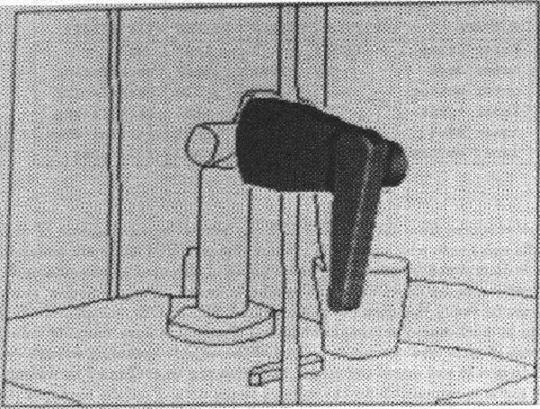
Figure 1.10 shows the predicted upper and lower arms at this angle.
was estimated
to be 4.57, compared to the measured value of 4.94.
Figure 1.10 shows the predicted upper and lower arms at this angle.
Missing features, such as the back of the trash can, are found by a model-directed process. Given the oriented model, the image positions of unmatched SURFACEs can be predicted. Then, any surfaces in the predicted area that:
Accounting for missing structure requires an understanding of the three cases of feature visibility, predicting or verifying their occurrence and showing that the image data is consistent with the expected visible portion of the model. The easiest case of back-facing and tangent SURFACEs can be predicted using the orientation estimates with known observer viewpoint and the surface normals deduced from the geometric model. A raycasting technique (i.e. predicting an image from an oriented model) handles self-obscured front-facing SURFACEs by predicting the location of obscuring SURFACEs and hence which portions of more distant SURFACEs are invisible. Self-occlusion is determined by comparing the number of obscured to non-obscured pixels for the front-facing SURFACEs in the synthetic image. This prediction also allows the program to verify the partially self-obscured SURFACEs, which were indicated in the data by back-side-obscuring boundaries. The final feature visibility case occurs when unrelated structure obscures portions of the object. Assuming enough evidence is present to invoke and orient the model, occlusion can be confirmed by finding closer unrelated surfaces responsible for the missing image data. Partially obscured (but not self-obscured) SURFACEs are also verified as being externally obscured. These SURFACEs are noticed because they have back-side-obscuring boundaries that have not been explained by self-occlusion analysis.
The self-occlusion visibility analysis for the trash can in the
scene is given in Table 1.3.
Minor prediction errors occur at edges where surfaces do not meet perfectly.
| SURFACE | VISIBLE PIXELS | OBSC'D PIXELS | TOTAL PIXELS | VISIBILITY |
|---|---|---|---|---|
| outer front | 1479 | 8 | 1487 | full |
| outer back | 1 | 1581 | 1582 | back-facing |
| outer bottom | 5 | 225 | 230 | back-facing |
| inner front | 0 | 1487 | 1487 | back-facing |
| inner back | 314 | 1270 | 1584 | partial-obsc |
| inner bottom | 7 | 223 | 230 | full-obsc |
Verifying missing substructure is a recursive process and is easy given the definition of the objects. Showing that the robot hand is obscured by the unrelated trash can decomposes to showing that each of the hand's SURFACEs are obscured.
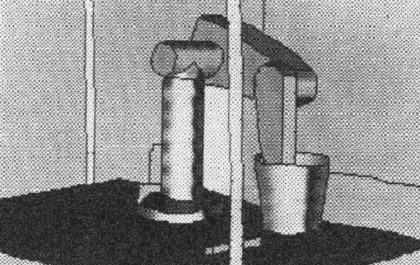
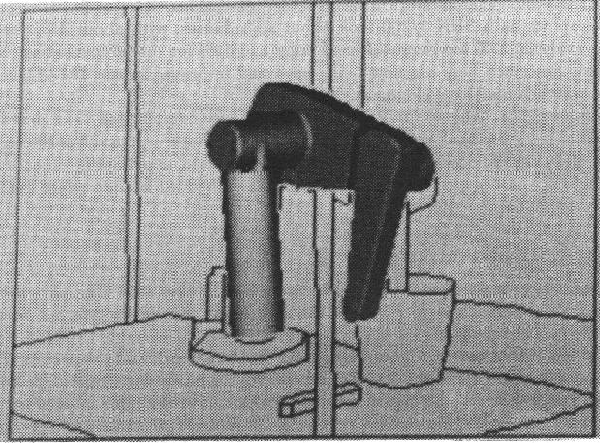
Figure 1.11 shows the found robot model as predicted by the orientation parameters and superposed over the original intensity image. Though the global understanding is correct, the predicted position of the lower arm is somewhat away from its observed position because of cumulative minor rotation angle errors from the robot's base position. In analysis, all features were correctly paired, predicted invisible or verified as externally self-obscured. The numerical results in Table 1.2 also show good performance.
The final step in the recognition process is verification (Chapter 10), which helps ensure that instantiated hypotheses are valid physical objects and have the correct identity. A proper, physical, object is more certain if all surfaces are connected and they enclose the object. Correct identification is more likely if all model features are accounted for, the model and corresponding image surface shapes and orientations are the same, and the model and image surfaces are connected similarly. The constraints used to ensure correct SURFACE identities were:
In the example given above, all correct object hypotheses passed these constraints. The only spurious structures to pass verification were SURFACEs similar to the invoked model or symmetric subcomponents.
To finish the summary, some implementation details follow. The IMAGINE I program was implemented mainly in the C programming language with some PROLOG for the geometric reasoning and invocation network compilation (about 20,000 lines of code in total). Execution required about 8 megabytes total, but this included several 256*256 arrays and generous static data structure allocations. Start-to-finish execution without graphics on a SUN 3/260 took about six minutes, with about 45% for self-occlusion analysis, 20% for geometric reasoning and 15% for model invocation. Many of the ideas described here are now being used and improved in the IMAGINE II program, which is under development.
The completely recognized robot is significantly more
complicated than previously recognized objects (because of its multiple
articulated features, curved surfaces, self-occlusion and external
occlusion).
This successful complete, explainable, object recognition was achieved
because of the rich information embedded in the surface
data and surface-based models.
Recognition Graph Summary
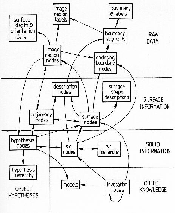
The recognition process creates many data structures, linked into a graph whose relationships are summarized in Figure 1.12. This figure should be referred to while reading the remainder of this book.
At the top of the diagram, the three bubbles "surface depth and orientation data", "image region labels" and "boundary and labels" are the image data input. The boundary points are linked into "boundary segments" which have the same label along their entire length. "Image region nodes" represent the individual surface image regions with their "enclosing boundary nodes", which are circularly linked boundary segments. "Adjacency nodes" link adjacent region nodes and also link to "description nodes" that record which boundary separates the regions.
The "image region nodes" form the raw input into the "surface nodes" hypothesizing process. The "surface nodes" are also linked by "adjacency nodes" and "enclosing boundary nodes". In the description phase, properties of the surfaces are calculated and these are also recorded in "description nodes". Surface shape is estimated and recorded in the "surface shape descriptors".
The surface cluster formation process aggregates the surfaces into groups recorded in the "surface cluster nodes". These nodes are organized into a "surface cluster hierarchy" linking larger enclosing or smaller enclosed surface clusters. The surface clusters also have properties recorded in "description nodes" and have an enclosing boundary.
Invocation occurs in a plausibility network of "invocation nodes" linked by the structural relations given by the "models". Nodes exist linking model identities to image structures (surface or surface cluster nodes). The invocation nodes link to each other to exchange plausibility among hypotheses.
When a model is invoked, a "hypothesis node" is created linking the model to its supporting evidence (surface and surface cluster nodes). Hypotheses representing objects are arranged in a component hierarchy analogous to that of the models. Image region nodes link to the hypotheses that best explain them.
This completes our overview of the recognition process and the following chapters explore the issues raised here in depth.