Surface Curvature

By the surface shape segmentation assumptions (Chapter 3), each surface region can be assumed to have constant curvature signs and approximately constant curvature magnitude. Using the orientation information, the average orientation change per image distance is estimated and this is then used to estimate absolute curvature. This description separates surface regions into curvature classes, which provides a first level of characterization. The absolute magnitude of the curvature then provides a second description.

Following Stevens [153] and others, the two principal curvatures, $\kappa_1$ and $\kappa_2$, are used to characterize the local shape of the surface (along with the directions of the curvatures). These are the maximum and minimum local curvatures of the planar curves formed by intersecting a normal plane with the surface. (The rotation angles at which these curvatures occur are orthogonal - a property that will be used later.) The signs of the two curvatures categorize the surfaces into six possible surface shape classes (Table 6.5). The curvature sign is arbitrary, and here convex surfaces are defined to have positive curvature.

Table 6.5: Surface Shape Classes

	$\kappa_1 < 0$	$\kappa_1 = 0$	$\kappa_1 > 0$
$\kappa_2 < 0$	CONCAVE ELLIPSOID	CONCAVE CYLINDER	HYPERBOLOID SURFACE
$\kappa_2 = 0$	CONCAVE CYLINDER	PLANE	CONVEX CYLINDER
$\kappa_2 > 0$	HYPERBOLOID SURFACE	CONVEX CYLINDER	CONVEX ELLIPSOID

Turner [161] classified surfaces into five different classes (planar, spherical, conical, cylindrical and catenoidal) and made further distinctions on the signs of the curvature, but here the cylindrical and conical categories have been merged because they are locally similar. Cernuschi-Frias, Bolle and Cooper [45] classified surface regions as planar, cylindrical or spherical, based on fitting a surface shading model for quadric surfaces to the observed image intensities. Both of these techniques use intensity data, whereas directly using the surface orientation data allows local computation of shape. Moreover, using only intensity patterns, the methods give a qualitative evaluation of shape class, instead of absolute curvature estimates. More recently, Besl [24] used the mean and gaussian curvature signs (calculated from range data) to produce a similar taxonomy, only with greater differentiation of the hyperboloidal surfaces.

Brady et al. [40] investigated a more detailed surface understanding including locating lines of curvature of surfaces and shape discontinuities using three dimensional surface data. This work gives a more accurate metrical surface description, but is not as concerned with the symbolic description of surface segments. Agin and Binford [5] and Nevatia and Binford [121] segmented generalized cylinders from light-stripe based range data, deriving cylinder axes from stripe midpoints or depth discontinuities.

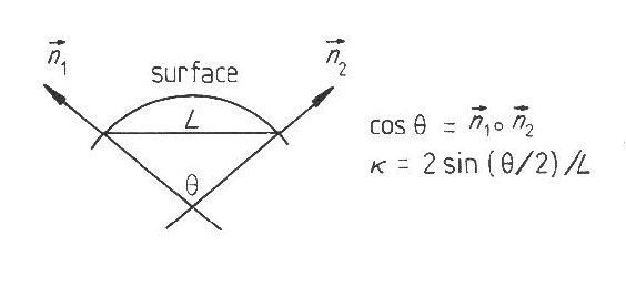
To estimate the curvature magnitude, we use the difference in the orientation of two surface normals spatially separated on the object surface. The ideal case of a cross-section perpendicular to the axis of a cylinder is shown in Figure 6.5. Two unit normals $\vec{n_1}$ and $\vec{n_2}$ are separated by a distance $L$ on the object surface. The angular difference $\theta$ between the two vectors is given by the dot product: $$\theta = arccos( \vec{n_1} \circ \vec{n_2} )$$

Then, the curvature estimate at this cross-section orientation is:

$$\kappa = 2 * sin( \theta / 2) / L$$

Figure 6.5: Surface to Chord Length Relationship

To find the two principal curvatures, the curvature at all orientations must be estimated. The planar case is trivial, and all curvature estimates are $\kappa = 0$.

Figure 6.6: Cross-Section Length Relationships

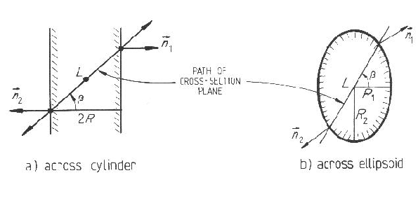
If the curvature is estimated at all orientations using the method above, then the minimum and maximum of these estimates are the principal curvatures. Part (a) of Figure 6.6 shows the path of the intersecting plane across a cylinder. For simplicity, assume that the orientation ($\beta$) of the plane intersecting the surface starts perpendicular to the axis of the cylinder. Further, assume that the cylinder surface is completely observed, so that the points at which the surface normals $\vec{n_1}$ and $\vec{n_2}$ are measured are at the extrema of the surface. Then, the normals are directly opposed, so that $\theta$ equals $\pi$ in the above expression. The curvature is then estimated for each orientation $\beta$. While the intersection curve is not always a circle, it is treated as if it is one.

Let $R$ be the cylinder radius. The chord length L observed at orientation $\beta$ is:

$$L = 2 * R / \mid cos(\beta) \mid$$

Hence, the curvature estimate (from above) is:

$$\kappa = 2 * sin( \theta / 2) / L = \mid cos(\beta) \mid / R$$

For the ellipsoid case (part (b) of Figure 6.6), the calculation is similar. Letting $R_1$ and $R_2$ be the two principal radii of the ellipsoid (and assuming that the third is large relative to these two) the length measured is approximately:

$$L = 2 * R_1 * R_2 / \sqrt{T}$$

where:

$$T = (R_1 * sin(\beta))^2 + (R_2 * cos(\beta))^2$$

Hence, the curvature estimate (from above) is:

$$\kappa = 2 * sin( \theta / 2) / L = \sqrt{T} / (R_1 * R_2)$$

The special case of the cylinder can be derived from this by looking at the limit as $R_2$ approaches infinity.

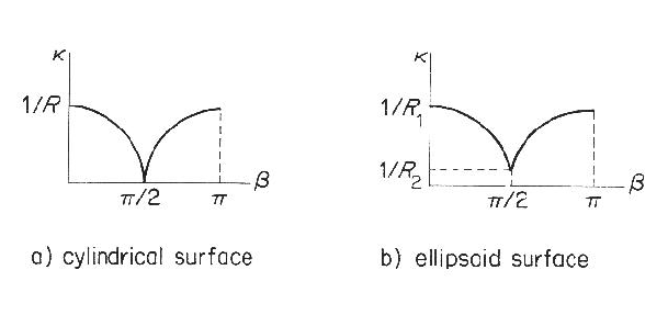
This analysis gives the estimated curvature versus cross-section orientation $\beta$. If $\beta$ is not aligned with a principal curvature axis, then the cross-section has a shifted phase. In any case, the minimum and maximum values of these estimates are the principal curvatures. The maximum curvature occurs perpendicular to the major curvature axis (by definition) and the minimum curvature occurs at $\pi / 2$ from the maximum. Figure 6.7 shows a graphical presentation of the estimated curvature versus $\beta$.

Figure 6.7: Ideal Estimated Curvature Versus Orientation

For simplicity, this analysis used the curvature estimated by picking opposed surface normals at the extremes of the intersecting plane's path. Real intersection trajectories will usually not reach the extrema of the surface and instead we estimate the curvature with a shorter segment using the method outlined at the beginning of this section. This produces different curvature estimates for orientations not lying on a curvature axis. However, the major and minor axis curvature estimates are still correct, and are still the maximum and minimum curvatures estimated. Then, Euler's relation for the local curvature estimated at orientations $\theta$ (not necessarily aligned with the principal curvatures) is exploited to find an estimate of the curvatures:

$$\kappa ( \beta ) = \kappa_1 * cos^2( \beta ) + \kappa_2 * sin^2( \beta) = \kappa_2 + (\kappa_1 - \kappa_2) * cos^2( \beta )$$

One might ask why the global separated normal vector approach to curvature estimation was used, rather than using derivatives of local orientation estimates, or the fundamental forms? The basis for this decision is that we wanted to experiment with using the larger separation to reduce the error in the orientation difference $\theta$ when dealing with noisy data. This benefit has to be contrasted with the problem of the curvature changing over distance. But, as the changes should be small by the segmentation assumption, the estimation should still be reasonably accurate. Other possibilities that were not tried were least-squared error fitting of a surface patch and fitting a curve to the set of normals obtained along the cross-section at each orientation $\beta$.

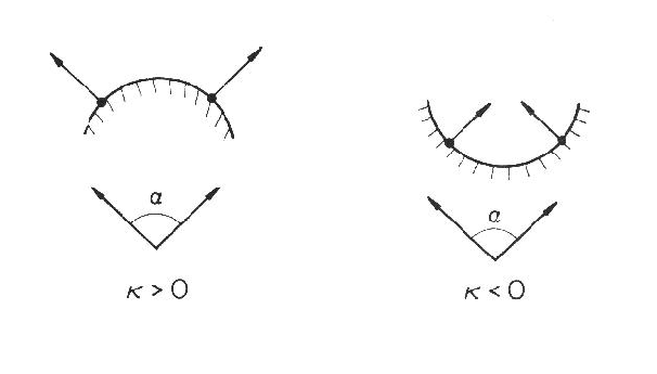
We now determine the sign of the curvature. As Figure 6.8 shows, the angle between corresponding surface normals on similar convex and concave surfaces is the same. The two cases can be distinguished because for convex surfaces the surface normals point away from the center of curvature, whereas for the concave case the surface normals point towards it.

Figure 6.8: Convex and Concave Surface Similarities

Given the above geometric analysis, the implemented surface curvature computation is:

1. Let $\vec{P}$ be a nominal point in the surface image region.
2. Generate the curvature estimate versus $\beta$ function as outlined above, for cross-sections through $\vec{P}$:
   1. find cross-section length $L$
   2. find surface orientation angle difference $\theta$
   3. estimate curvature magnitude $\mid \kappa \mid$
3. Fit $cos^2( \alpha )$ to the curvature versus $\beta$ function to smooth estimates and determine the phase angle.
4. Extract maximum and minimum curvature magnitudes.
5. At maximum and minimum curvature orientations, check direction of surface normal relative to surface.
   1. if towards the center, then $\kappa < 0$
   2. if away from the center, then $\kappa > 0$

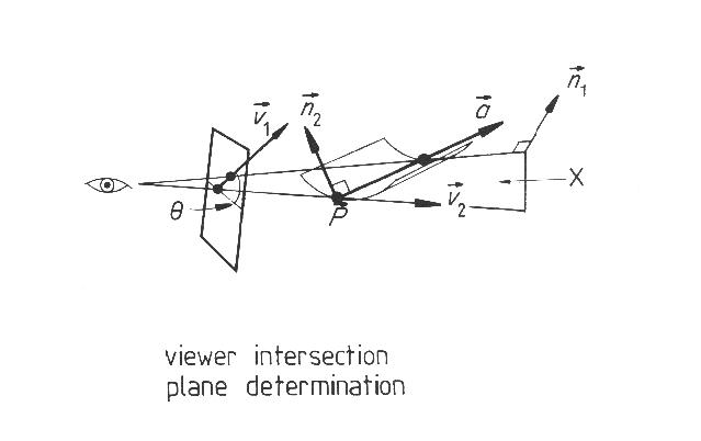
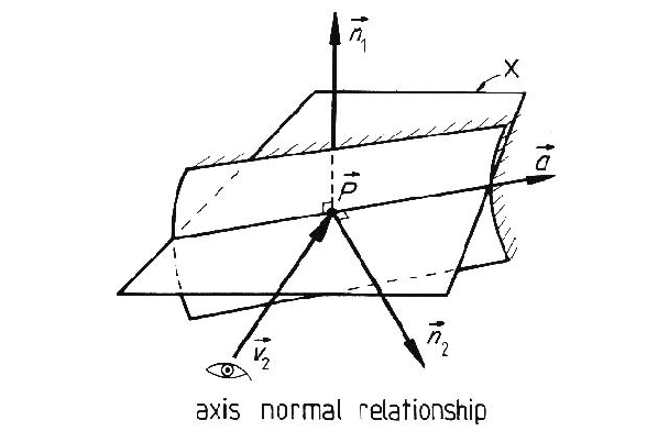
The estimation of the major axis orientation for the surface region is now easy. (The major axis is that about which the greatest curvature occurs.) The plane case can be ignored, as it has no curvature. Figures 6.9 and 6.10 illustrate the geometry for the axis orientation estimation process.

Figure 6.9: Curvature Axis Orientation Estimation (Find Axis Plane)

Figure 6.10: Curvature Axis Orientation Estimation (Find Vector)

We calculate the axis direction by calculating the direction of a parallel line $\vec{a}$ through the nominal point $\vec{P}$. We start by finding a plane X that this line lies in (see Figure 6.9). Plane X contains the viewer and the nominal point $\vec{P}$. Hence, the vector $\vec{v_2}$ from the viewer to the nominal point lies in the plane. Further, we assume that line $\vec{a}$ projects onto the image plane at the image orientation $\theta$ at which the minimum curvature is estimated. Hence, the vector $\vec{v_1} = (cos( \theta ),sin( \theta ),0)$ also lies in plane X. As the two vectors are distinct ($\vec{v_1}$ is seen as a line, whereas $\vec{v_2}$ is seen as a point), the normal $\vec{n_1}$ to plane X is:

$$\vec{n_1} = \vec{v_1} \times \vec{v_2}$$

Line $\vec{a}$ lies in this plane (see Figure 6.10) so it must be perpendicular to the plane's normal $\vec{n_1}$. It is also perpendicular to the surface normal $\vec{n_2}$. Hence, the direction of line $\vec{a}$ is:

$$\vec{a} = \vec{n_1} \times \vec{n_2}$$

This vector is used as an estimate of the major curvature axis direction. The minor curvature axis direction is given by $\vec{a} \times \vec{n_2}$.

The curvature and axis orientation estimation process was applied to the test scene. The curvatures of all planar surfaces were estimated correctly as being zero. The major curved surfaces are listed in Tables 6.6 and 6.7, with the results of their curvature and axis estimates. (If the major curvature is zero in Table 6.6, then the minor curvature is not shown.) In Table 6.7, the error angle is the angle between the measured and estimated axis vectors.

Table 6.6: Summary of Surface Curvature Estimates

IMAGE REGION	MAJOR(MJ) MINOR(MN)	ESTIMATED CURVATURE	TRUE CURVATURE
8	MJ	.11	.11
	MN	0	0
9	MJ	.09	.08
	MN	0	0
12	MJ	0	0
16	MJ	.15	.13
	MN	0	0
18	MJ	0	0
25	MJ	.19	.13
	MN	0	0
26	MJ	0	0
29	MJ	.12	.13
	MN	0	0
31	MJ	.07	.09
	MN	0	0

Table 6.7: Summary of Curved Surface Curvature Axis Estimates

IMAGE REGION	ESTIMATED AXIS	TRUE AXIS	ERROR ANGLE
8	(0.0,0.99,-0.1)	(0.0,1.0,0.0)	0.10
16	(-0.99,0.0,0.0)	(-0.99,0.0,0.1)	0.09
25	(-0.99,0.07,0.11)	(-0.99,0.0,0.1)	0.13
31	(-0.86,-.21,-0.46)	(-0.99,0.0,0.1)	0.53
9	(-0.09,0.99,-0.07)	(0.0,1.0,0.0)	0.12
29	(-.14,0.99,0.0)	(0.0,1.0,0.0)	0.14

The estimation of the surface curvature and axis directions is both simple and mainly accurate, as evidenced by the above discussion and the results. The major error is on the small, nearly tangential surface (region 31), where the curvature estimates are acceptable, but the algorithm had difficulty estimating the orientation, as might be expected. Again, as the depth and orientation estimates were acquired by hand, this is one source of error in the results. Another source is the inaccuracies caused by interpolating depth and orientation estimates between measured values.

The major weak point in this analysis is that the curvature can vary over a curved surface segment, whereas only a single estimate is made (though the segmentation assumption limits its variation). Choosing the nominal point to lie roughly in the middle of the surface helps average the curvatures, and it also helps reduce noise errors by giving larger cross-sections over which to calculate the curvature estimates.