The properties that we would like invocation to have are:
Three minor analytic results have been found:
(1) If all property, subcomponent, description and superclass evidence is perfect, then the correct model is always invoked. This is equivalent to saying that the object has the correct identity and all properties are measured correctly. If we then assume the worst (i.e. that the other four evidence types are totally contradictory) then evidence integration gives:
| Let: | |
|
|
|
|
|
|
| be the eight evidence values | |
| Then, following the integration computation: | |
|
|
|
|
|
|
|
|
|
|
|
|
|
|
|
| and the integrated plausibility value |
|
|
|
|
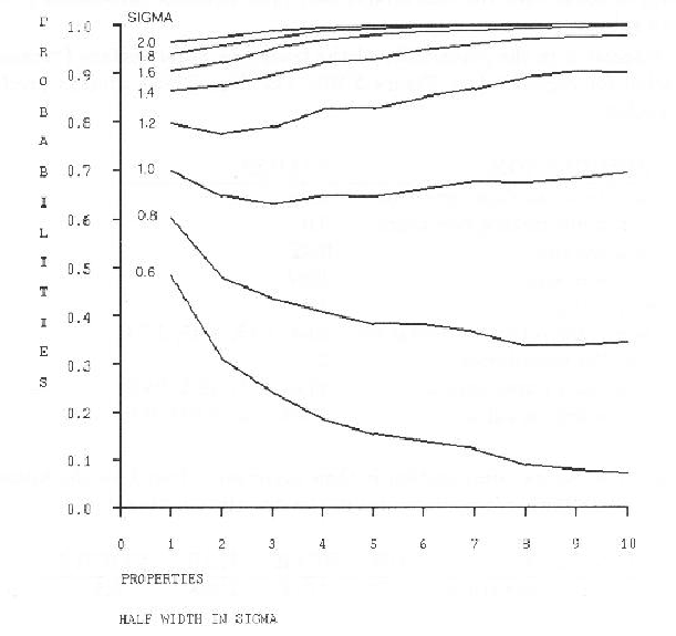
(2) Assume ![]() independent properties are measured as property evidence for
a structure, and all are equally weighted.
Then, the probability that the property evidence evaluation is greater than zero
is shown in Figure 8.13, assuming all constraint ranges have the widths
shown, and the data values are normally distributed.
The point is to estimate how many properties are needed and what the constraint
ranges on a property should be, to ensure that the property evidence almost
always supports the correct identity.
The graph shows that if at least 5 gaussian distributed properties are
used, each with constraint width of at least 1.6 standard deviations, then there
is a probability of 0.98 for positive property evidence.
These results were found by simulation.
independent properties are measured as property evidence for
a structure, and all are equally weighted.
Then, the probability that the property evidence evaluation is greater than zero
is shown in Figure 8.13, assuming all constraint ranges have the widths
shown, and the data values are normally distributed.
The point is to estimate how many properties are needed and what the constraint
ranges on a property should be, to ensure that the property evidence almost
always supports the correct identity.
The graph shows that if at least 5 gaussian distributed properties are
used, each with constraint width of at least 1.6 standard deviations, then there
is a probability of 0.98 for positive property evidence.
These results were found by simulation.
(3) There is some relative ranking between the same model in different
contexts:
model ![]() has better evidence in context
has better evidence in context ![]() than in context
than in context ![]() if, and only if
if, and only if
![]() .
Further, if model
.
Further, if model ![]() implies model
implies model ![]() (i.e. a superclass), then
in the same context
(i.e. a superclass), then
in the same context ![]() :
:
The theory proposed in this chapter accounts for and integrates many of the major visual relationship types. The surface cluster contexts focus attention to ASSEMBLY identities (and surface contexts to SURFACE identities), the object types denote natural conceptual categories, and the different relationship links structure the paths of evidence flow. The mathematical results suggest that "correct models are always invoked" if the data is well-behaved.
The "no false invocations" requirement is not easily assessed without a formal definition of "similar", and none has been found that ensures that false invocations are unlikely. So, a performance demonstration is presented, using the model base partly shown in Appendix A with the test image, and show that the invocation process was effective and robust.
Suppose interest is in the plausibility of the trash can outer surface
("tcanoutf") as an explanation for region 9 (see Figure 3.10).
The description process produces the following results:
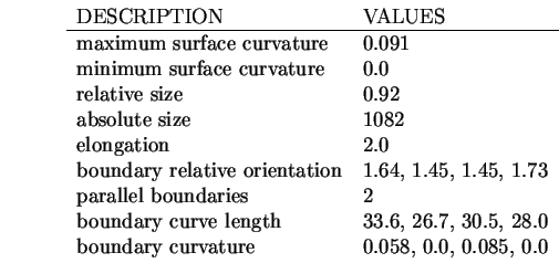
The property evidence computation is then performed, based on the
following evidence constraint (all other properties are in the description
"tcanfac"):

This results in a property evidence value of 0.74 with weight 0.5. After invocation converges, there are also the relationship evidence values. No subclasses, superclasses, subcomponents or associations were defined for this model, so their evidence contribution is not included. The model has a description "tcanfac" that shares properties of the trash can inner surface ("tcaninf") except for its convexity or concavity, and its evidence value is 0.66 with a weight of 5.3. The supercomponent evidence value is 0.38 because "tcanoutf" belongs to the trash can ASSEMBLY. The maximum of the other SURFACE plausibility values for non-generically related identities is 0.41 (for the "robbodyside" model), so this causes inhibition. These evidence values are now integrated to give the final plausibility value for "tcanoutf" as 0.62. As this is positive, the trash can outer surface model will be invoked for this region.
We now consider the problem of invoking the trash can ASSEMBLY model in
surface cluster 8 (from Table 5.1), which is composed of
exactly the trash can's outer and inner surface regions.
For each of the two surfaces, three possible identities
obtain: trash can inner surface, trash can outer surface
and trash can bottom.
The trash can model specifies only subcomponent and inhibition relationships and
defines three subcomponents:
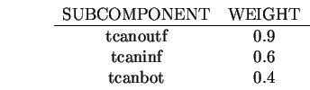
    SUBCGRP OF trashcan = tcanoutf tcaninf;
    SUBCGRP OF trashcan = tcanoutf tcanbot;
    SUBCGRP OF trashcan = tcaninf tcanbot tcanoutf;
The plausibilities of the subcomponent model SURFACE instances are:
| DATA INNER | DATA OUTER | |
| MODEL INNER | -0.42 | 0.26 |
| MODEL OUTER | -0.48 | 0.62 |
| MODEL BOTTOM | -0.81 | -0.88 |
The subcomponent evidence computation starts with the best plausibility for each model feature: inner = 0.26, outer = 0.62, bottom = -0.81. (Note that, because of occlusion, the data outer surface provides better evidence for the model inner SURFACE that the data inner surface, because all properties other than maximum curvature are shared. This does not cause a problem; it only improves the plausibility of the inner SURFACE model.) The visibility group calculation used the harmonic mean with the weightings given above to produce a subcomponent evidence value of 0.46, -0.08 and 0.01 for the three visibility groups. Finally, the best of these was selected to give the subcomponent evidence of 0.46.
The highest competing identity was from the robbody model, with a plausibility of 0.33. Integrating these evidence values gives the final plausibility for the trash can as 0.38, which was the supercomponent plausibility used in the first example.
Because there are far too many plausibility and evidence values to describe
the whole network, even for this modest model base (16 ASSEMBLYs,
25 SURFACEs, and 24 generic descriptions: 22 for SURFACEs and 2 for ASSEMBLYs), we next present a
photograph of the network to illustrate the general character of the computation, and then
look at the invoked model instances in more detail.
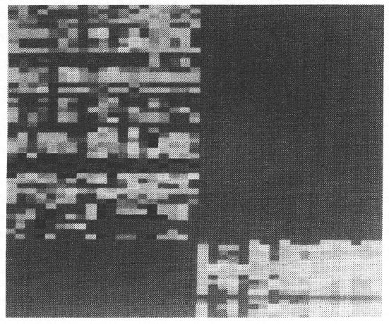
Figure 8.14 shows all model instance nodes of the network in
its converged state.
In the large region at the upper left of the picture (with the textured
appearance) each small grey colored rectangle represents one model instance.
The brightness of the box encodes its plausibility,
from black (![]() ) to white (
) to white (![]() ).
The model instances are represented in a two dimensional grid, indexed
by the image features
horizontally from left-to-right with surfaces first and then the surface clusters.
The vertical index lists the model features from top to bottom, with
model SURFACEs and then ASSEMBLYs.
The two large black areas on the upper right and lower left arise from type
incompatibility
(model SURFACEs with surface clusters on the upper right and ASSEMBLYs
with image surfaces on the lower left).
The cover jacket of the book shows the results of the network more clearly, by
encoding the plausibility from blue (
).
The model instances are represented in a two dimensional grid, indexed
by the image features
horizontally from left-to-right with surfaces first and then the surface clusters.
The vertical index lists the model features from top to bottom, with
model SURFACEs and then ASSEMBLYs.
The two large black areas on the upper right and lower left arise from type
incompatibility
(model SURFACEs with surface clusters on the upper right and ASSEMBLYs
with image surfaces on the lower left).
The cover jacket of the book shows the results of the network more clearly, by
encoding the plausibility from blue (![]() ) to red (
) to red (![]() ).
).
Several interesting features can be seen immediately. First, there is a strong horizontal grouping of black and white boxes near the middle of the upper left surface pairing nodes. These are for the generic description evidence types, such as planar, positive cylinder, etc. As they are defined by only a few properties, they achieve strong positive or negative plausibilities. The specific model SURFACEs are above, and other generic SURFACE features are below these. Only the specific model SURFACEs can be invoked, and there are only a few bright-grey to white nodes with a plausibility that is high enough for this, whereas there are many darker grey low plausibility nodes (more details below).
A similar pattern is seen in the ASSEMBLY nodes on the lower right, except for a large brightish region on the right side, with many potentially invokable model instances. This bright region occurs because: (1) there are several nested surface clusters that all contain much of the robot and (2) a surface cluster containing most of an object generally acquires a high plausibility for the whole object. This led to the explicit disabling of model instance nodes after verification, as described previously.
All invocations for this image are summarized in Tables 8.1 and 8.2 (surface clusters are listed in Table 5.1 and image regions are shown in Figure 3.10). As commented above, successful invocations in one context mask invocations in larger containing contexts. Further, generic models are not invoked - only the object-specific models. Hence, not all positive final plausibilities from Figure 8.14 cause invocation.
ASSEMBLY invocation is selective with 18 invocations of a possible 288 (16 ASSEMBLY models in 18 surface cluster contexts). Of these, all appropriate invocations occur, and nine are in the smallest correct context and one is in a larger context. Of the others, three are justified by close similarity with the actual model (note 1 in the table) and five are unjustified (notes 2 and 3).
SURFACE model invocation results are similar, with 21 invocations
out of 475 possible (25 SURFACE models in 19 surface contexts).
Of these, ten were correct, five are justifiably incorrect because
of similarity (note 1) and six are inappropriate invocations (notes
2 and 3).
| MODEL | SURFACE CLUSTER | PLAUSIBILITY | INVOCATION STATUS | NOTES |
|---|---|---|---|---|
| robshldbd | 3 | 0.50 | E | |
| robshldsobj | 5 | 0.45 | E | |
| robshldsobj | 2 | 0.44 | I | 2 |
| robshldsobj | 11 | 0.44 | I | 2 |
| robshould | 11 | 0.39 | E | |
| trashcan | 8 | 0.38 | E | |
| robbody | 12 | 0.33 | I | 1 |
| robbody | 13 | 0.33 | I | 1 |
| robbody | 8 | 0.33 | I | 1 |
| robbody | 15 | 0.33 | L | |
| lowerarm | 7 | 0.29 | E | |
| link | 15 | 0.15 | E | |
| robot | 14 | 0.14 | I | 3 |
| robot | 15 | 0.14 | E | |
| link | 17 | 0.11 | I | 3 |
| armasm | 13 | 0.09 | E | |
| upperarm | 9 | 0.05 | E | |
| robot | 17 | 0.02 | I | 3 |
| STATUS | |
|---|---|
| E | invocation in exact context |
| L | invocation in larger than necessary context |
| I | invalid invocation |
| NOTES | |
| 1 | because true model is very similar |
| 2 | ASSEMBLY with single SURFACE has poor discrimination |
| 3 | not large enough context to contain all components |
| MODEL | SURFACE REGION | PLAUSIBILITY | INVOCATION STATUS | NOTES |
|---|---|---|---|---|
| robshldend | 26 | 0.76 | C | |
| tcanoutf | 9 | 0.61 | C | |
| robbodyside | 9 | 0.41 | I | 1 |
| robshoulds | 29 | 0.40 | C | |
| robshoulds | 27 | 0.40 | I | 3 |
| ledgea | 18 | 0.36 | C | |
| lendb | 31 | 0.27 | C | |
| tcaninf | 9 | 0.26 | I | 1 |
| ledgeb | 18 | 0.25 | I | 1 |
| robshould1 | 16 | 0.21 | I | 1 |
| robshould2 | 16 | 0.21 | C | |
| lsidea | 12 | 0.20 | I | 1 |
| lsideb | 12 | 0.20 | C | |
| robbodyside | 8 | 0.11 | C | |
| robshould1 | 12 | 0.10 | I | 3 |
| robshould2 | 12 | 0.10 | I | 3 |
| uside | 19,22 | 0.07 | C | |
| uedgeb | 19,22 | 0.07 | I | 2 |
| lsidea | 19,22 | 0.04 | I | 2 |
| lsideb | 19,22 | 0.04 | I | 2 |
| uends | 25 | 0.02 | C |
| STATUS | |
|---|---|
| C | correct invocation |
| I | invalid invocation |
| NOTES | |
| 1 | because of similarity to the correct model |
| 2 | because the obscured correct model did not inhibit |
| 3 | because of some shared characteristics with the model |
Clearly, for this image, the invocation process works well. The chief causes for improper invocation were: