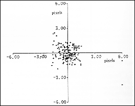
Figure 9: Back projected image plane errors after calibration of the full 4 DOF head system.


The epi-polar constraint is one of the most fundamentally useful pieces of information which can be exploited during stereo matching. It can be shown by elementary geometry [1] that 3D feature points are constrained to lie along epi-polar lines in each image. Knowledge of the epi-polars reduces the correspondence problem to a 1D search. This constraint is best utilised by the process of image rectification. The principle is quite simple, any pair of images can be transformed to a "parallel camera geometry" so that corresponding point features in 3D will lie on the same horizontal line in the two images. Unfortunately such a process requires some knowledge of the left to right camera transformation which will generally require a calibration proceedure. The freedom for camera model specification, cost function definition and numerical implementation is immense. It is perhaps somewhat unfortunate that the subject must continue to be a drain on research efforts during the development of new systems. Camera calibration is quite a Pandoras box of publications and methods ( the most commonly referenced text is probably [12] ) but a few guidelines can be provided as to what constitutes good practice.
The camera model must be specified with a minimum number of parameters which describe the important degrees of freedom. There are at least three ways of representing the left-to-right camera coordinate rotation matrix. The quaternion, the screw (Rodriegez method) and polar co-ordinate triple axis rotation, there is probably very little to distinguish between the performance of these methods. If the cameras display radial distortion effects these may well not be visible to the casual observer but will weaken the accuracy of the epi-polar constraint and completely bias any resulting 3D measurement. Image centres and aspect ratios may also need to be free parameters and can generally not be expected to take default (side of the box) values.
The cost function must be defined in the image plane as the errors between back projected positions for points. This is the only domain in which measurement errors can be expected to be uniform so that systematic errors are not introduced during the calibration process. If the data for calibration is to be obtained from any automatic matching process then the cost function must be in the form of a robust statistic. Any automatic calibration proceedure which is based on least-squares will be susceptible to calibration matching failiures and must be viewed with suspiscion.
A practical calibration system must give some indication of resulting calibration accuracy, either in terms of resulting back projected error or as covariance estimates on the estimated parameters. Ideally any subsequent stereo algortihm should be capable of interpreting these measures and adjusting output depth accuracy estimates accordingly.
A recent focus of research has been in the area of "self-calibration", the rational being that it is possible to calibrate cameras from the data available during use rather than having to rely on special purpose calibration data. This is an admirable endevour but all of these techniques must be evaluated on the basis of the above criteria if they are to form the basis of a reliable automatic system. Unfortunately, numerical robustness is often sacrificed for mathematical sophistication.
Optimal techniques for robust combination of fixed camera calibration have been used to fuse data from robot motion, matched stereo corner correspondances and a calibration tile. The accuracy of estimated epipolar geometry was found to improve with the inclusion of new data as expected [9]. This system supports online recalibration of a variable verge stereo camera system using data from the fixed verge calibration method over a relatively large range of rotations.
The pan/tilt and left verge parameters were obtained by calibrating on the back projected robot motion and matched static 3D points. The resulting full camera model was tested on unseen robot positions (Figure 9) Outliers can be seen which are generated by several causes including stereo mis-matching and undershoot of the robot arm. This parameterisation of the system now permits 3D data from different head configurations to be combined into one coordinate frame and computation of head configurations for fixation of 3D world points.

Figure 9: Back projected image plane errors after calibration of the full
4 DOF head system.


