Experiments

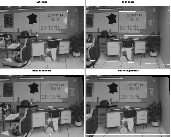
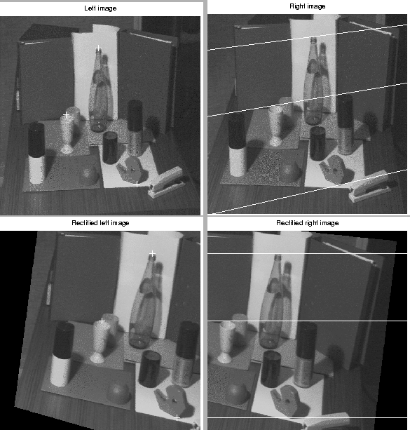
For this experiments we used calibrated stereo pairs from INRIA-Syntim. We show the results obtained with a nearly rectified stereo rig (Figure 3) and with a more general stereo geometry (Figure 4). The pixel coordinates of the rectified images are not constrained to lie in any special part of the image plane, and an arbitrary translation were applied to both images to bring them in a suitable region of the plane, by changing the image center. Then the output images were cropped to the size of the input images.

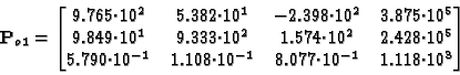
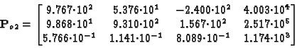
For example, In the case of the ``Sport'' stereo pair (image size $768 \times 576$), we started from the following camera matrices:

$${\bf P}_{o1} = \begin{bmatrix} 9.765{\cdot}10^2 & 5.382{\cdo... ...10^{-1} & 8.077{\cdot}10^{-1} & 1.118{\cdot}10^3 \end{bmatrix}$$

$${\bf P}_{o2} = \begin{bmatrix}9.767{\cdot}10^2 & 5.376{\cdot}... ...}10^{-1} & 8.089{\cdot}10^{-1} & 1.174{\cdot}10^3 \end{bmatrix}$$

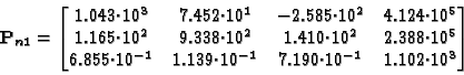
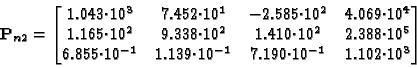
After adding the statement A(1,3) = A(1,3) + 160
to the rectify program, to keep the rectified image in the center of the $768 \times 576$ window, we obtained the following rectified camera matrices:

$${\bf P}_{n1} = \begin{bmatrix} 1.043{\cdot}10^3 & 7.452{\cdo... ...10^{-1} & 7.190{\cdot}10^{-1} & 1.102{\cdot}10^3 \end{bmatrix}$$

$${\bf P}_{n2} = \begin{bmatrix} 1.043{\cdot}10^3 & 7.452{\cdo... ...0^{-1} & 7.190{\cdot}10^{-1} & 1.102{\cdot}10^3 \end{bmatrix}$$

  

Figure 3: ``Sport'' stereo pair (top) and rectified pair (bottom). The right pictures plot the epipolar lines corresponding to the points marked in the left pictures.

  

Figure 4: ``Color'' stereo pair (top) and rectified pair (bottom). The right pictures plot the epipolar lines corresponding to the points marked in the left pictures.