


Imagine a grey-scale image; for example, two concentric rings of differing
grey values. Choosing a threshold value of  is clearly
inappropriate, since the value ``between'' the two rings may not
straddle the value of
is clearly
inappropriate, since the value ``between'' the two rings may not
straddle the value of  , as it would it an original binary image.
Instead, our goal is to locally construct an appropriate thresholding
value. We follow the philosophy of the algorithm for binary images.
, as it would it an original binary image.
Instead, our goal is to locally construct an appropriate thresholding
value. We follow the philosophy of the algorithm for binary images.
Imagine a grey scale image, such as the two concentric rings, in which
the inner ring is slightly darker then the exterior ring;
here, we interpret this as  being more negative in the interior
ring than the exterior.
Furthermore, imagine a slight notch protruding outwards into the
lighter ring, (see Figure 9).
Our goal is decide whether the area within the notch belongs to the
lighter region, that is, whether it is a perturbation that should
be suppressed and "reabsorbed" in to the appropriate background color.
We determine this by first computing the average value of the
intensity
being more negative in the interior
ring than the exterior.
Furthermore, imagine a slight notch protruding outwards into the
lighter ring, (see Figure 9).
Our goal is decide whether the area within the notch belongs to the
lighter region, that is, whether it is a perturbation that should
be suppressed and "reabsorbed" in to the appropriate background color.
We determine this by first computing the average value of the
intensity  in the neighborhood around the point.
We then must determine a comparison value which indicates the
``background'' value.
We do so by computing a threshold
in the neighborhood around the point.
We then must determine a comparison value which indicates the
``background'' value.
We do so by computing a threshold  , defined as
the average value of the intensity obtained
in the direction perpendicular to the gradient direction. Note that since
the direction perpendicular to the gradient is tangent to the
isointensity contour through
, defined as
the average value of the intensity obtained
in the direction perpendicular to the gradient direction. Note that since
the direction perpendicular to the gradient is tangent to the
isointensity contour through  , the two points used to compute
are either in the same region, or the point
, the two points used to compute
are either in the same region, or the point  is an inflection point,
in which the curvature is in fact zero and the min/max flow will always
yield zero.
is an inflection point,
in which the curvature is in fact zero and the min/max flow will always
yield zero.
Formally then,
This has the following effect. Imagine again our case of a grey
disk on a lighter grey background, where the darker grey corresponds to
a smaller value of  than the lighter grey. When the threshold is
larger than the average, the max is selected, and the level curves
move in. However, as soon as the average becomes larger, the min switch
takes over, and the flow stops. The arguments are similar to the ones
given in the binary case.
than the lighter grey. When the threshold is
larger than the average, the max is selected, and the level curves
move in. However, as soon as the average becomes larger, the min switch
takes over, and the flow stops. The arguments are similar to the ones
given in the binary case.
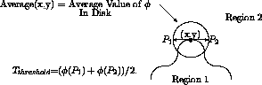
Figure 9: Threshold Test for Min/Max Flow
In Figure 10, we use this scheme to remove salt-and-pepper
gray-scale noise from a grey-scale image. Once again, we add noise to
the figure by replacing  of the pixels with a new value, chosen
from a uniform random distribution between 0 and 255,
Our results are obtained as follows. We begin with two levels of
noise;
of the pixels with a new value, chosen
from a uniform random distribution between 0 and 255,
Our results are obtained as follows. We begin with two levels of
noise;  noise in Figure 10a and
 noise in Figure 10d.
We first use the min/max flow from Eqn.13 until a
steady-state is reached in each case, (Figure 10b and
Figure 10e).
This removes most of the noise. We then continue with a larger
stencil for the threshold to remove further noise
(Figure 10c and Figure 10f). For the larger stencil,
we computer the average
noise in Figure 10d.
We first use the min/max flow from Eqn.13 until a
steady-state is reached in each case, (Figure 10b and
Figure 10e).
This removes most of the noise. We then continue with a larger
stencil for the threshold to remove further noise
(Figure 10c and Figure 10f). For the larger stencil,
we computer the average  over a larger disk, and compute the
threshold value
over a larger disk, and compute the
threshold value  using a correspondingly longer tangent
vector.
using a correspondingly longer tangent
vector.
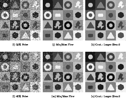
Figure 10: Min/Max Flow. The left column is the original with noise, the
center column is the steady-state of min/max flow, the right column is
the continuation of the min/max flow using a larger stencil
