A note on image encoding

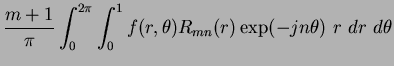
By returning to the continuous form of the Zernike moments (in order to enable easy manipulation of the moments), it is possible to gain an insight into the image encoding itself. As before, the Zernike moments are defined by Equation 1.49, where the Zernike polynomials are expressed by Equation 1.51. Converting the integration of Equation 1.49 to polar coordinates, using $dx~dy= r~dr~d\theta$ and Equations 1.51, 1.56 and 1.57, produces:

$$A_{mn} = \frac{m+1}{\pi}\int_{x}\int_{y} f(x,y) [V_{mn}(x,y)]^*~dx~dy ~~~~~\mbox{where $x^{2} + y^{2} \leq ~1$}$$

$$= \frac{m+1}{\pi} \int_0^{2\pi}\int_0^1 f(r,\theta)R_{mn}(r)\exp(-jn\theta)~r~ dr~d\theta$$ (61)

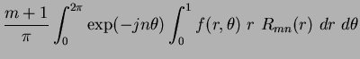
Re-arranging the integral produces:

$$A_{mn} = \frac{m+1}{\pi} \int_0^{2\pi} \exp(-jn\theta) \int_0^1 f(r,\theta)~ r~R_{mn}(r)~dr~d\theta$$ (62)

It can be seen that the $f(r,\theta)$ term is weighted by $r R_{mn}(r)$. The radial polynomials are normalised such that:

$$R_{mn}(1) = 1$$ (63)

is true [3,9]. Due to the unit disc, $r$ is at a maximum when equal to unity, meaning that:

$$\mid R_{mn}(r)\mid \leq 1$$ (64)

This result is illustrated in Figure 1.6. Using these results and returning to the weighted term (in Equation 1.62), we can see that the weighting is bounded by $r$:

$$\mid r R_{mn}(r) \mid \leq r$$ (65)

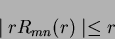
This produces descriptions which are weighted in favour of their distance from the origin of the unit disc. Those pixels lying closer to the perimeter of the unit disc will have more weight than those lying closer to the origin. As $r$ approaches unity the radial polynomials display steeper gradients and converge (becoming more correlated - Figures 1.6 and 1.7). The higher order polynomials (and their corresponding moments) will have improved capability in describing image detail due to their increased oscillations (see Figure 1.7) especially in the region before convergence due to the increased frequency of these oscillations. Image detail which is encoded around the region of convergence will be more correlated. However, these characteristics can be exploited. Considering the case of applied perimeter noise on simple shapes (i.e. circle, square and triangle), the effects of the noise (close to the disc's perimeter) can be reduced by scaling the shape (during mapping) to an appropriate size, where the noise cannot be described efficiently enough to pose a problem, however enabling sufficient detail to describe the shape.

Figure 1.7: Higher order orthogonal radial polynomial plotted for increasing $r$.