Next: Relating Zernike and Cartesian
Up: Orthogonal moments
Previous: A note on image
Image reconstruction
The method of moment matching (Section 1.2.3), as described for the reconstruction of non-orthogonal moments is also applicable to reconstruction of an image by orthogonal moments. However, the orthogonality condition enables a faster, more direct approach.
Teague [18] showed that, for orthogonal Legendre moments, if all moments of a Cartesian function  up to a given order
  are known, then it is possible to reconstruct a discrete function
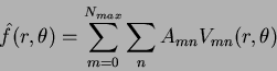
  , whose moments match those of the original function , up to the order . This relationship is due to the orthogonality condition of the Legendre moments, while the accuracy of the reconstructed function improves as approaches infinity. Khotanzad [7] expressed this relationship in terms of Zernike moments, shown here in radial coordinates:
 |
(66) |
and  is constrained by Equation 1.50.
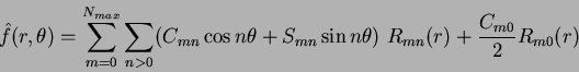
Expanding this using real-valued functions produces:
is constrained by Equation 1.50.
Expanding this using real-valued functions produces:
 |
(67) |
composed of their real (![$Re[.]$](img227.png) ) and imaginary (
) and imaginary (![$Im[.]$](img228.png) ) parts:
) parts:
bounded by  . Here, each Zernike moment simply adds its own contribution to the function
 , unlike the Cartesian reconstruction case discussed in Section 1.2.3.
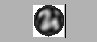
Figure 1.8b shows the result of order
, unlike the Cartesian reconstruction case discussed in Section 1.2.3.
Figure 1.8b shows the result of order  through
  reconstruction on a
  image, while Figure 1.8a is the original image. Orders
  and
and  are discarded due to the scale and translation mapping used, Equations 1.58 and 1.59. This makes
 zero, while
 (the shape's area) is set to a known value,
  .
Due to the nature of the function
, the Gibbs phenomena [16] will affect the final result (as already mentioned for the moment matching case in Section 1.2.3). However, the effects are less apparent in Figure 1.8b due to faster convergence of the final function
.
.
Due to the nature of the function
, the Gibbs phenomena [16] will affect the final result (as already mentioned for the moment matching case in Section 1.2.3). However, the effects are less apparent in Figure 1.8b due to faster convergence of the final function
.
Next: Relating Zernike and Cartesian
Up: Orthogonal moments
Previous: A note on image
Jamie Shutler
2002-08-15
![$\displaystyle 2 Re\left[A_{mn}\right] = \frac{2m+2}{\pi} \sum_x \sum_y f(r,\theta) R_{mn}(r) \cos n\theta$](img230.png)
![$\displaystyle -2 Im\left[A_{mn}\right] = \frac{-2m-2}{\pi} \sum_x \sum_y f(r,\theta) R_{mn}(r) \sin n\theta$](img232.png)