Orthogonal moments

Cartesian moments, Equation 1.13 are formed using a monomial basis set $x^{p}y^{q}$. This basis set is non-orthogonal and this property is passed onto the Cartesian moments. These monomials increase rapidly in range as the order increases, producing highly correlated descriptions. This can result in important descriptive information being contained within small differences between moments, which leads to the need for high computational precision.

However, moments produced using orthogonal basis sets exist. These orthogonal moments have the advantage of needing lower precision to represent differences to the same accuracy as the monomials. The orthogonality condition simplifies the reconstruction of the original function from the generated moments. Orthogonality means mutually perpendicular, expressed mathematically - two functions $y_m$ and $y_n$ are orthogonal over an interval $a\leq x\leq b$ if and only if:

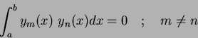$$\int_{a}^{b}y_m(x)~y_n(x) dx = 0~~~;~~~m\neq n$$ (44)

Here we are primarily interested in discrete images, so the integrals within the moment descriptors are replaced by summations. It is noted that a sequence of polynomials which are orthogonal with respect to integration, are also orthogonal with respect to summation, [21]. Two such (well established) orthogonal moments are Legendre and Zernike.