Next: Symmetry properties
Up: Non-orthogonal moments
Previous: Centralised moments
Image reconstruction
Having described an image by a set of moments, it may prove useful to investigate which moments give rise to which characteristics of the image, or vice versa. This can be achieved by reconstructing the original image from the calculated moments.
Moment reconstruction, for moments with orthogonal basis functions (such as Legendre and Zernike
moments which will be discussed later) has been developed extensively, [11,12,18,19].
However, where the basis set is non-orthogonal (such as Cartesian and centralised moments),
only one method has appeared (although, non-orthogonal transform methods exist). This is the method of moment matching for non-orthogonal moment
reconstruction [18]. The method is based upon creating a continuous
function that has identical moments to that of the original function. In this section it has been applied first
to Cartesian moments and then to the centralised moments. It must be noted that
in applying the theory to sampled images, the continuous conditions are replaced by discrete versions,
reducing the accuracy of the final function.
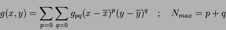
Assuming that all moments  of a function
  and of order
  are known from zero
through to order
are known from zero
through to order  , it is then possible to obtain the continuous function
  whose
moments match those of the original function , up to order . (With reference to the Taylor series expansion in Section 1.1), assuming that the given
continuous function can be defined as:
whose
moments match those of the original function , up to order . (With reference to the Taylor series expansion in Section 1.1), assuming that the given
continuous function can be defined as:
 |
(22) |
which reduces to:
 |
(23) |
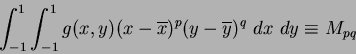
then the constant coefficients  , are calculated, so that the moments of match those
of , assuming that the image is a continuous function bounded by:
, are calculated, so that the moments of match those
of , assuming that the image is a continuous function bounded by:
![\begin{displaymath}
x~\epsilon~[-1,1]~~,~~y~\epsilon~[-1,1]
\end{displaymath}](img87.png) |
(24) |
These limits can be achieved by normalising the pixel range over which the Cartesian moments are calculated, thus:
 |
(25) |
Substituting Equation 1.22 into Equation 1.25 and then solving the integration produces a
set of Linear Equations (LE), the number of which is determined by the order  of
reconstruction. These can then be solved for the coefficients (in terms of the moments
) by using matrix inversion. For order three (
of
reconstruction. These can then be solved for the coefficients (in terms of the moments
) by using matrix inversion. For order three ( ), the LEs in matrix form are:
![\begin{displaymath}
\left[ \begin{array}{*{3}{c}}
\hspace*{0.5cm} & \hspace{0.5...
...{*{1}{c}}
M_{00} \\
M_{20} \\
M_{02} \\
\end{array} \right]
\end{displaymath}](img90.png) |
(26) |
![\begin{displaymath}
\left[ \begin{array}{*{3}{c}}
\hspace*{0.5cm} & \hspace{0.5...
...{*{1}{c}}
M_{10} \\
M_{30} \\
M_{12} \\
\end{array} \right]
\end{displaymath}](img91.png) |
(27) |
![\begin{displaymath}
\left[ \begin{array}{*{3}{c}}
\hspace*{0.5cm} & \hspace{0.5...
...{*{1}{c}}
M_{01} \\
M_{03} \\
M_{21} \\
\end{array} \right]
\end{displaymath}](img92.png) |
(28) |
and finally:
 |
(29) |
Applying matrix inversion to the first matrix, Equation 1.26 produces:
![\begin{displaymath}
\left[ \begin{array}{*{3}{c}}
\hspace*{0.5cm} & \hspace{0.5...
...{*{1}{c}}
g_{00} \\
g_{20} \\
g_{02} \\
\end{array} \right]
\end{displaymath}](img94.png) |
(30) |
By repeating this for all the matrices, it is possible to calculate all the coefficients. If they are then
substituted back into Equation 1.22
an expression for is produced. This expression can then used to reconstruct an approximation
of the
original image. The reconstruction function is now in terms of weighted sums of the moments
, which have been previously calculated from the original function . The resultant
function for order three is:
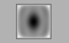
Implementing this method to order  for binary images of simple
shapes produces recognisable results, as shown in Figures 1.3 and
1.4.
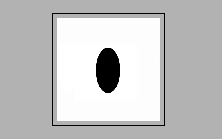
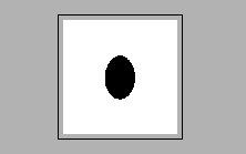
Figure 1.3a is the original image from which the moments were calculated
and Figure 1.3b is the image reconstructed from the moments. The borders
of the shape appear unclear, but they appear when the reconstructed image is thresholded,
Figure 1.3c.
Here the level of the applied threshold was adjusted by visual comparison with the original image.
Due to the nature of the continuous function, the final shape is dependent on the threshold level, as is apparent in Figure 1.3c, as compared with the original image, Figure 1.3a.
for binary images of simple
shapes produces recognisable results, as shown in Figures 1.3 and
1.4.
Figure 1.3a is the original image from which the moments were calculated
and Figure 1.3b is the image reconstructed from the moments. The borders
of the shape appear unclear, but they appear when the reconstructed image is thresholded,
Figure 1.3c.
Here the level of the applied threshold was adjusted by visual comparison with the original image.
Due to the nature of the continuous function, the final shape is dependent on the threshold level, as is apparent in Figure 1.3c, as compared with the original image, Figure 1.3a.
Figure 1.3:
Order  Cartesian reconstruction of an ellipse.
   |
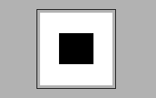
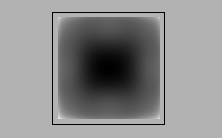
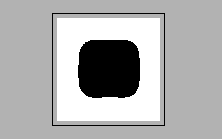
This analysis is then repeated for the rectangle in Figure 1.4.
The corners of the rectangle in Figure 1.4c are missing. The corners represent the high frequency content in the image, thus will be described fully by higher order moments. So the thresholded shape will converge to the original shape as the number of moments (and thus the order) increases. However for more complex shapes, higher accuracy
 is needed. This is analogous to the high frequency information needed to reconstruct
pulsed time domain waveforms, using methods like Fourier series.
As the order (and accuracy) increases, so does the number of LEs that need
to be solved (reconstruction for order eight resulted in
forty five LE's). Further, if it was required to increase the order of reconstruction (using Equation 1.31), then all coefficients need to be re-calculated. This is due to the correlated nature of the Cartesian moments, each moment does not simply provide its own individual contribution, (unlike the orthogonal case which will be discussed later in this chapter).
It is interesting to note the effects of the Gibbs phenomena [16] which are more evident in the reconstructed ellipse - Figure 1.3b. The Gibbs phenomena (explained in terms of Fourier series) is the inability for a continuous function to recreate a step function - no matter how many finite high order terms are used, an overshoot of the function will occur. Here the discontinuous edge of the original intensity function of the ellipse (between the ellipse and the background) appear unclear in the reconstruction. While outside of the original area of the ellipse, `ripples' of overshoot of the continuous function are visible.
is needed. This is analogous to the high frequency information needed to reconstruct
pulsed time domain waveforms, using methods like Fourier series.
As the order (and accuracy) increases, so does the number of LEs that need
to be solved (reconstruction for order eight resulted in
forty five LE's). Further, if it was required to increase the order of reconstruction (using Equation 1.31), then all coefficients need to be re-calculated. This is due to the correlated nature of the Cartesian moments, each moment does not simply provide its own individual contribution, (unlike the orthogonal case which will be discussed later in this chapter).
It is interesting to note the effects of the Gibbs phenomena [16] which are more evident in the reconstructed ellipse - Figure 1.3b. The Gibbs phenomena (explained in terms of Fourier series) is the inability for a continuous function to recreate a step function - no matter how many finite high order terms are used, an overshoot of the function will occur. Here the discontinuous edge of the original intensity function of the ellipse (between the ellipse and the background) appear unclear in the reconstruction. While outside of the original area of the ellipse, `ripples' of overshoot of the continuous function are visible.
By assuming the same constraints as for Cartesian moment matching, the theory can be
extended to centralised moments. The continuous function is now defined as:
 |
(32) |
similarly, Equation 1.25 becomes:
 |
(33) |
where  and
and  are the
  and
and  COM's, respectively.
Solving for is then achieved in the same manner as already described for the Cartesian case.
COM's, respectively.
Solving for is then achieved in the same manner as already described for the Cartesian case.
Next: Symmetry properties
Up: Non-orthogonal moments
Previous: Centralised moments
Jamie Shutler
2002-08-15