Next: Non-orthogonal moments
Up: Statistical moments - An
Previous: Statistical moments - An
The moment generating function
To describe the distribution of a random variable the characteristic function can be used [10]:
![\begin{displaymath}
X(w) = \int_{-\infty}^{\infty} f(x) \exp(jwx)~dx = E[\exp(jwx)] %%\sum_E P(E)\exp(iwE)
\end{displaymath}](img18.png) |
(4) |
shown here for the signal density  , where
  and
and  is the spatial frequency.
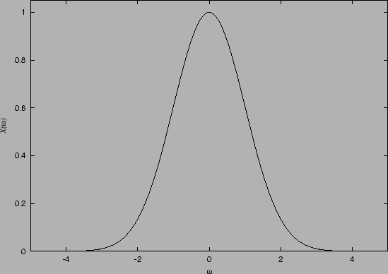
This is essentially the Fourier transform of the signal and has a maximum at the origin
is the spatial frequency.
This is essentially the Fourier transform of the signal and has a maximum at the origin  , as
, as  . Figure 1.1 shows an example of
  for a zero mean, unit variance Gaussian density .
Figure 1.1:
Characteristic function of a Gaussian density .
 |
If One dimensional continuous functionis the density of a positive, real valued random variable  , such that
 , then a continuous exponential distribution can be defined. Replacing
  in Equation 1.4 with
  produces a real valued integral of the form:
![$\displaystyle M^x(s) = \int_{-\infty}^{\infty} f(x) \exp(xs)~dx = E[\exp(xs)]$](img28.png) |
|
|
(5) |
where ![$E[.]$](img29.png) is the expectation and
is the expectation and  exists as a real number. is called the moment generating function, shown here for a one-dimensional distribution.
It is used to characterise the distribution of an ergodic signal.
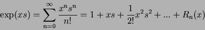
Expressing the exponential in terms of an expanded Taylor series produces:
exists as a real number. is called the moment generating function, shown here for a one-dimensional distribution.
It is used to characterise the distribution of an ergodic signal.
Expressing the exponential in terms of an expanded Taylor series produces:
 |
(6) |
where  is the error term. It can be seen that the series will only converge and represent
  completely if
  . Therefore, if the distribution is finite in length, all values outside this length must be zero (or in terms of an image, all values outside the sampled image plane must be zero). Assuming this and substituting Equation 1.6 into Equation 1.5 produces:
where  is the
  moment about the origin.
Differentiating Equation 1.5
moment about the origin.
Differentiating Equation 1.5  times with respect to produces:
![\begin{displaymath}
M^x_n(s) = E[x^n\exp(xs)]
\end{displaymath}](img43.png) |
(8) |
If is differentiable at zero, then the order moments about the origin are given by:
![\begin{displaymath}
M^x_n(0) = E[x^n] = m_n
\end{displaymath}](img44.png) |
(9) |
So the first three moments of this distribution are:
If the distribution of the signal is a Gaussian, then it is completely described by its two moments, mean ( ) and variance (
 ), while the total area (
 ) is
) is  .
If the joint moment
.
If the joint moment  for two signals is required (i.e. a two-dimensional image) then it is noted that:
![\begin{displaymath}
M^{xy}(s) = E[ \exp((x+y)s)] = E[ \exp(xs)\exp(ys)] %%\nonumber \\
\end{displaymath}](img56.png) |
(11) |
and assuming that and  are independent, then:
![\begin{displaymath}
M^{xy}(s) = E[ \exp(xs)] E[ \exp(ys)] = M^x(s)M^y(s)
\end{displaymath}](img57.png) |
(12) |
In conclusion, it is possible to evaluate the moments of a distribution by two methods. Either by using the direct integration (Equation 1.1), or by use of the moment generating function (Equation 1.5). However, in practice the moment generating function is more widely applied to the problem of calculating moment invariants, while the direct integration method is used to calculate specific moment values.
Next: Non-orthogonal moments
Up: Statistical moments - An
Previous: Statistical moments - An
Jamie Shutler
2002-08-15