Experiments

To compare the different representations, we use a standard histogram recognition scheme [27]. Although this does not take into account the spatial arrangement of an image, it is useful in identifying CVs of objects, since it gives a good indication of the stability of a representation to small changes of viewpoint. The behaviour of the different measures under the histogram recognition procedure enables qualitative assessment of the representations in terms of average CV extent.

We measure the proximity between two images using the Bhattacharyya distance

$$B(P_Q,P_M)={- \ln {\displaystyle \sum_{i=1}^n \sqrt{P_Q(i) \times P_M(i)} } }$$

where P_Q is the query histogram and P_M one of the model histograms.

Figure 2 illustrates the results of our experiments for 4 of the 20 images in the test set. This image set is the Columbia Image Object Library, consisting of 20 arbitrary objects. There are 72 views of each object, illuminated by a light source coincident with the camera. The images are taken at $5^{\circ}$ intervals along a great circle of the object's view-sphere. Only around 9% of the view-sphere is spanned by these 72 images, underlining the need for view grouping if appearance-based object recognition is not to require unfeasibly large numbers of models.

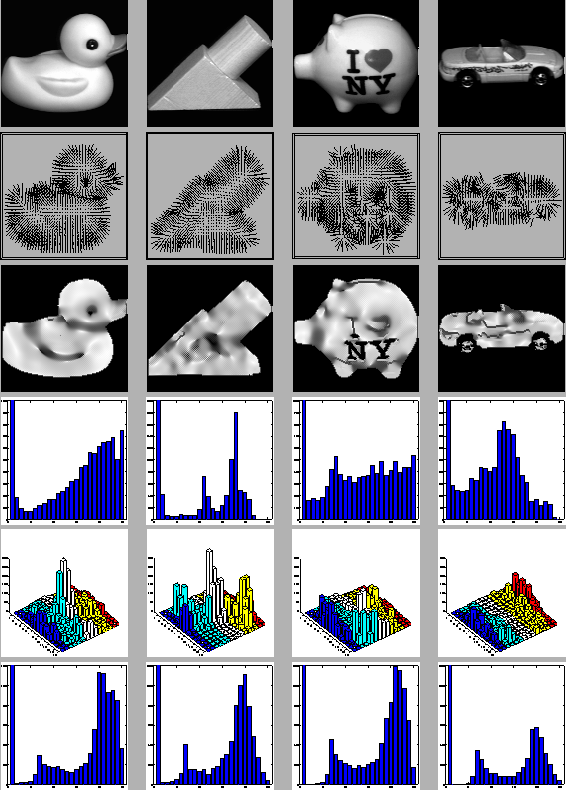
The first row of Figure 2 shows the first image from each of the 72 view sequences for 4 objects in the dataase. The second row shows the needle-maps recovered by the SFS technique described in Section 2, whilst the third row displays the shape index classes derived from the needle-map. The grey-levels correspond to the scale in Figure 1.

Rows 4-6 of Figure 2 show the histograms for each of the object representations in turn. In each case, the leftmost bin corresponds to background pixels and is excluded from the calculation of Bhattacharyya distance between the histograms.

Row 4 shows the grey-level histograms for the raw images, and Row 5 the 2-D histograms of the needle-maps. Clearly, there is a great deal of variability in the structure of these 2-D histograms.

The shape-index histograms of Row 6 are all broadly similar. Each is bi-modal, with the two modes corresponding approximately to ruts and ridges/domes.

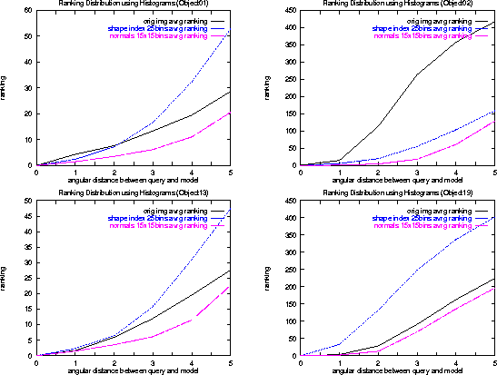
Figure 3 shows histogram ranking results for each of the representations. These are average plots taken over all 72 images representing a given object. In each case, one of the 72 images is chosen as the query image, and all 1440 images in the database ranked according to their distance from this query. Clearly, the query image itself has zero self-distance and hence is ranked 0. Views of the same object from similar viewpoints, i.e. those with small angular deviations in any direction on the viewsphere, should come next in the ranking, and so on. Each image in the set representing a given object is taken as the query in turn, and an average ranking found for all images at a given angular distance either side of the query. This is repeated for each of the object representations.

To establish CVs, we require a representation which provides a good ranking ability over as wide a range of angular distance as possible. The surface normal representation clearly meets this requirement in each of the cases shown. Specifically, it provides a better ranking ability over a wider range of angular distances than the raw images. The shape-index also does relatively well for the first two objects, but is unstable to even small changes in viewing angle for the second pair of objects. The latter images contain significant surface markings, resulting in rapid changes of albedo. These break the fundamental Lambertian assumptions underlying our SFS technique, leading to poor needle-map recovery in these regions. The recovery errors are subsequently compounded in the calculation of the shape-index.

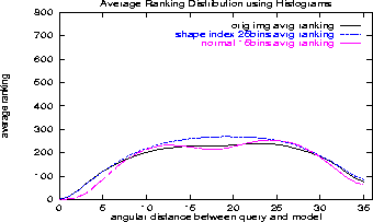
Figure 4 shows the averaged ranking results, over the full $\pm 180^{\circ }$ range of angular distances. Here we display the result of taking each of the 1440 images as the query image in turn and averaging the rankings of all images of the same object as the query. The results are plotted as a function of the angular distance from the query. We use only one bin size for each representation. The shape-index does poorly in comparison to the raw intensity images. However, there is a clear advantage in using the needle-map as the average ranking remains much lower over a wider range of angular distances from the query image.

  

Figure 2: Top row: Raw Images. Row 2: Recovered Needle-maps. Row 3: Shape Index representation. Row 4: 25 bin grey-level frequency histograms. Row 5: 15x15 bin 2-D histograms of normal direction frequency. Row 6: 25 bin shape index frequency histograms.

  

Figure: Plots of average ranking vs distance from query over all images of a given object. Each one of the 72 images of the object is taken as the query image in turn, and all 1440 images in the database ranked according to their distance from this query. The average ranking found for all images at a given angular distance either side of the query. An angular distance of 1 represents the average of the images at $\pm 5^{\circ }$ from the query.

  

Figure: Plots of average ranking vs distance from query over all images in the database. Each of the 1440 images is taken as the query image in turn. The dip around angular distance 18 ( $\pm 90^{\circ }$), and the larger dip towards angular distance 35 ( $\pm 180^{\circ }$), are attributable to a number of the objects possessing approximate rotational symmetry of order 2 and 4 respectively.